6 Understanding Effect Size and Power in Psychological Research
In psychological research, understanding not just whether a difference exists, but also how large that difference is, is crucial. This chapter will explore two key concepts that help us do this: effect size and statistical power. Effect size measures the magnitude of a relationship or the difference between groups, providing insight into the practical significance of findings. Statistical power, on the other hand, refers to the likelihood that a study will detect an effect when there is one. Together, these concepts allow us to draw more meaningful conclusions from our data, moving beyond simple yes-or-no answers provided by statistical significance.
By the end of this chapter and the associated exercise, you will understand how to calculate and interpret effect sizes, how to consider the power of a study before data collection begins, and why these factors are just as important—if not more so—than the p-value traditionally used in hypothesis testing.
6.1 Real-World Example of Effect Size and Power
Imagine a scenario where a psychologist is comparing the effectiveness of two types of therapy for reducing anxiety: Cognitive Behavioural Therapy (CBT) and Mindfulness-Based Stress Reduction (MBSR). After conducting a study, they find a statistically significant difference between the two therapies in terms of their impact on anxiety levels.
This is where understanding effect size comes in. Effect size will tell us how big the difference between CBT and MBSR is. If the effect size is large, it suggests that one therapy is meaningfully better than the other, and this difference could have important implications for treatment decisions. However, if the effect size is small, even though the difference is statistically significant, it might not be practically important.
Now, consider statistical power. If the study had a small sample size, the power might be low, meaning there was a higher chance of not detecting a difference even if one existed. In contrast, a study with high power reduces the risk of missing a true effect, giving more confidence in the results.
In the following sections we’ll look at these concepts in detail, how they are calculated and how we can use those calculations to build on our existing statistical findings.
6.2 What is Effect Size?
While p-values tell us whether there is evidence of an effect, effect size represents the magnitude or strength of such an effect. It provides a way to understand the practical significance of research findings by indicating the size of the difference between groups or the strength of the relationship between variables. In essence, effect size helps us move beyond asking, "Is there difference?" to answering, "How big is the difference?"
Effect size can be measured in several ways, depending on the type of data and the nature of the analysis. Below are some of the most commonly used effect size measures in psychological research.
6.2.1 Cohen’s d
Cohen’s d is one of the most widely used measures of effect size. It quantifies the difference between the means of two groups in terms of standard deviations. For instance, if we were comparing the average anxiety levels of participants receiving CBT versus those receiving MBSR, Cohen’s d would tell us how much these groups differ, relative to the variability within each group. - Small Effect (d ~0.2): A small effect size indicates a modest difference between groups, often noticeable only under certain conditions or in large samples. - Medium Effect (d ~ 0.5): A medium effect size suggests a moderate difference, generally visible and meaningful in most contexts. - Large Effect (d ~ 0.8): A large effect size indicates a substantial difference, easily noticeable and likely to be of practical importance.
Below is an illustration of these different effect sizes:
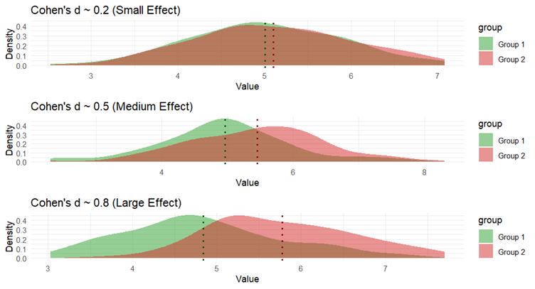
Each of the three graphs represents how data from each group is spread out. Think of it as a smoothed version of a histogram (a graph that shows where most of the data points are). The x-axis (horizontal) shows the possible values that participants score, and the y-axis (vertical) shows how likely participants are to score such a score.
In each graph, the green area represents "Group 1," and the red area represents "Group 2." The dotted lines show the average (mean) value for each group.
The less the two areas overlap the greater the difference between the two groups and the greater the effect size.
A interactive version of this image can be seen in the automatic t-test generator that I shared in the previous chapter: Automatic t-test generator
6.2.2 How is Cohen’s d calculated?
You’ll likely calculate Cohen’s d with a single click of a box in JASP or other statistical software, but it’s helpful to understand where this number comes from and what it represents. So, let’s break down how Cohen’s d is calculated.
Cohen’s d measures the difference between the means of two groups, relative to the variability within those groups. It’s essentially a way of standardising the difference so that it is possible to compare findings across different studies, even if they used different scales or measurements.
Here’s the basic formula:
\[ d = \frac{M_1 - M_2}{SD_{pooled}} \]
Where:
\(M_1\) and \(M_2\) are the means (averages) of the two groups.
\(SD_{pooled}\) is the pooled standard deviation of the two groups, which is a measure of the spread or variability of the data.
6.2.3 Breaking it Down:
-
Difference in Means
- First, we calculate the difference between the mean values of the two groups. This tells us how far apart the groups are on whatever measure you’re using (e.g. anxiety scores).
-
Pooled Standard Deviation
- Pooled SD is a bit more complex, but in simple terms, it’s an average of the standard deviations of the two groups. It gives us a sense of how spread out the scores are in each group.
- The formula for the pooled standard deviation is:
\[ SD_{pooled} = \sqrt{\frac{(n_1 - 1) SD_1^2 + (n_2 - 1) SD_2^2}{n_1 + n_2 - 2}} \]
Where:
\(SD_1\) and \(SD_2\) are the standard deviations of each group.
\(n_1\) and \(n_2\) are the sample sizes of each group.
This part of the formula adjusts for the fact that the groups might have different variabilities or different numbers of participants.
Finally, we divide the difference in means by the pooled standard deviation. This gives us Cohen’s d, which tells us how big the difference is in standard deviation units.
And, as mentioned previously, Cohen’s d can be interpreted as:
Small effect when d is roughly 0.2 or lower. The minimum value is 0.
Medium effect when d is roughly 0.5
Large effect when d is roughly 0.8 or higher. There is no upper bound, however, if the effect size is above around 2.0, I’d take that as an indication that I’d done something wrong in the analysis or data entry/cleaning as no meaningful, well-designed experiment should have a difference that big.
6.3 Other Measures of Effect Size
Cohen’s d is not the only measure of effect size. In fact, Cohen’s d is mostly just used in t-test comparisons.
Later in this book we will talk about Eta-Squared (η²) and Partial-Eta Squared (η²p). These are used primarily in ANOVA (Analysis of Variance), but the principle is much the same (with just a slightly different interpretation of the values).
We will also be looking at r and R-squared in the regression section of this book, these are the correlational equivalent of effect size measurement.
6.4 Effect Size Meaning Recap
Understanding effect size is critical because it goes beyond statistical significance to address the real-world implications of research findings. A p-value might tell us that a difference between groups is unlikely to be due to chance, but it doesn't tell us if that difference is large enough to be meaningful.
For example, in a large study, even a tiny difference might yield a significant p-value. However, if the effect size is small, this difference might not be important in practical terms. Conversely, a large effect size in a smaller study could indicate a very meaningful difference, even if it doesn't yield statistical significance due to a small sample size.
In psychological research, reporting effect size allows for a better understanding of the magnitude of findings and facilitates comparison across studies. It also aids in meta-analyses, where effect sizes from different studies are combined to assess the overall strength of a phenomenon. By considering both statistical significance and effect size, researchers can provide a fuller, more nuanced interpretation of their results, leading to more informed decisions in both research and practice.
For a deeper understanding of effect size see Lakens, D. (2022). Improving Your Statistical Inferences. Section 6.1 – 6.6
6.5 Overview of Statistical Power
Statistical power is a crucial concept in psychological research that is closely related to effect size. While effect size tells us the magnitude of a difference, statistical power tells us how likely we are to detect that magnitude of a difference if that difference actually exists.
Understanding statistical power is essential in the planning and design stages of your research, as it directly influences the decision on how many participants are needed in a study. Given that participant recruitment can be both costly and time-consuming, assuring adequate power will make sure your study is sensitive enough to detect meaningful differences, while reducing the risk of overlooking important effects.
6.5.1 Recap of type I and type II error
When you conduct a study in psychology, the evidence you collect to test your hypotheses is almost guaranteed not to be a perfect representation of reality. Your measures won’t be perfect, your manipulations might be fallible, your participants are unlikely to be truly representative of your population, and/or countless other confounding factors.
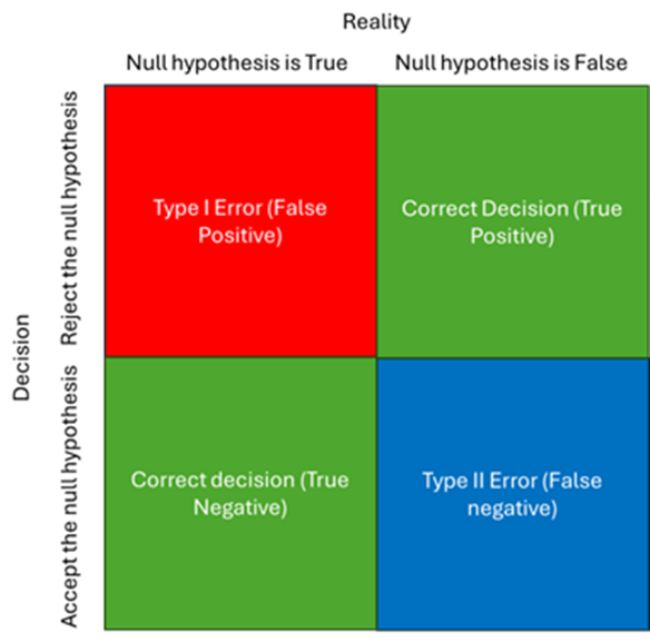
As such, it’s best to think in terms of there being four possible outcomes to your research:
- You find evidence of a difference, and this difference is a reliable reflection of the difference found in reality (True Positive)
- You find no evidence of a difference, and this difference is a reliable reflection of the difference found in reality (True Negative)
- You find evidence of a difference, however, in reality there is no difference (false positive, Type I error)
- You find no evidence of a difference, however, in reality there is a difference (false negative, Type II error)
A good way to think of this concept is to pretend that you are a judge in a court case. Your role is to decide guilt or innocence based on the evidence presented to you. Underlying that decision is the knowledge that if the evidence is unreliable, you may be convicting an innocent person or letting a guilty person go free.
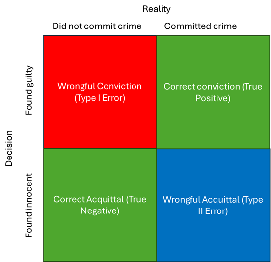
Our job in science, just as in the legal system, is to minimize the likelihood of Type I and Type II errors while increasing the chance of correctly identifying the true nature of reality.
Imagine now that the grid is the full set of possible outcomes from our experiment. Conducting an experiment is much like throwing a dart at this grid. If we start with the simplistic view that each box has an equal area, we’d have a 25% chance of hitting each one of the boxes—meaning there's a 50% chance of our experiment working as designed (landing in the "correct decision" boxes) and a 50% chance of giving an answer that is not representative of reality (landing in one of the error boxes). This scenario illustrates a poorly designed experiment with no mechanisms in place to improve our odds.
6.5.2 Reducing Type I Errors:
To improve our chances, we need to adjust the likelihood of each outcome. You’ve already encountered one key way we reduce Type I errors: setting an alpha level. In psychology, we typically accept a false positive rate (Type I error) of 5%. This means we are willing to risk concluding that there is an effect (when there isn’t) 5% of the time. In practice, this is controlled by the p-value, which tells us the probability of observing the data (or something more extreme) if the null hypothesis were true. If the p-value falls below the threshold of 0.05 (which represents 5%, or 1 in 20), we reject the null hypothesis, accepting a small chance that we're making a Type I error.
6.5.3 Addressing Type II Errors:
Now, let's consider Type II errors—where we fail to detect a true effect. Unlike Type I errors, which are controlled by setting the alpha level, Type II errors are influenced by the power of the study. Power is the probability of correctly rejecting the null hypothesis when it is false (i.e., avoiding a Type II error). The higher the power, the less likely we are to miss a true effect.
In psychology, we generally aim for a power of 0.80, meaning there is an 80% chance that our study will detect a true effect if one exists, leaving a 20% chance of making a Type II error.
Together this is how the hypothetical grid will typically look for a psychology study under the above criteria.
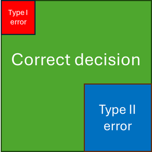
In psychological research, we are generally stricter with Type I errors than Type II errors because the consequences of a false positive (Type I error) are often considered more serious. A Type I error means concluding that an effect or difference exists when it actually does not, which can lead to false theories, wasted resources, and potentially harmful applications in practice, such as the adoption of ineffective treatments. By setting a low alpha level (commonly 0.05), we aim to minimize the risk of making such incorrect claims. While Type II errors (false negatives) are also important, they are often viewed as less critical because they imply that we missed an existing effect, which can be corrected with further research. In contrast, the propagation of a false positive can have far-reaching and lasting impacts on both science and practice. Again, think in terms of convicting an innocent person as compared to not convicting a guilty person.
6.6 Power Analysis
Power analysis helps us determine the necessary sample size for our study to achieve a desired level of power. By conducting a power analysis before collecting data, we can estimate how many participants we need to reliably detect an effect of a given size. The analysis takes into account the alpha level, the effect size we expect, and the desired power.
For example, if we expect a small effect size, we would need a larger sample to achieve 80% power than we would if we expected a large effect size. Without a sufficient number of participants, our study might be underpowered, increasing the risk of a Type II error.
In the next chapter I walk you through how to conduct an a-priori power analysis for an independent samples t-test. And later in this book we’ll return to the concept to illustrate how you can plan your intended sample size for more complex studies.
For a deeper understanding of effect size see Lakens, D. (2022). Improving Your Statistical Inferences. Section 8
In the next chapter we will run though how to conduct a power analysis for your study design.