8 Introduction to ANOVA
ANOVA, which stands for Analysis of Variance, is a statistical test used when comparing a continuous dependent variable across three or more groups. While it might seem similar to the t-test you've already learnt about, there is a fundamental issue that needs to be overcome when we move from two groups to more than two groups.
In this chapter we will learn about the basic one-way ANOVA, a design with a single independent variable with 3 or more levels, before moving on to factorial ANOVA, a design with more than one independent variable, in the next chapter.
This lecture chunk gives an overview of the ANOVA family of tests:
8.1 Example of a one-way ANOVA design
Imagine a study designed to investigate how to best frame an information campaign to prepare residence of a local area for an extreme weather event. In this experiment, participants are randomly assigned to one of four levels of an independent variable (i.e. a between subjects design).
Messaging (independent variable):
Fear-Based Messaging: Messages that emphasise the severe consequences of not being prepared.
Efficacy-Based Messaging: Messages that focus on practical steps individuals can take and highlight their ability to effectively prepare.
Community-Focused Messaging: Messages that highlight the importance of collective preparedness and how working together can improve community resilience.
Control condition: No message
Preparedness (Dependent variable): - Measured using a scale developed for the study. Scored from 0 to 100, with higher scores indicating greater intentions to engage in preparedness behaviours, such as creating an emergency kit or making a family plan.
Hypothesis:
H1: It is hypothesised that the type of preparedness messaging will significantly affect participants' intentions to prepare for disasters.
H2: Efficacy-based messaging is expected to generate the highest preparedness intentions, followed by community-focused messaging, fear-based messaging generating the lowest intentions.
H3: All forms of messaging will lead to higher preparedness than the control, no messaging, condition.
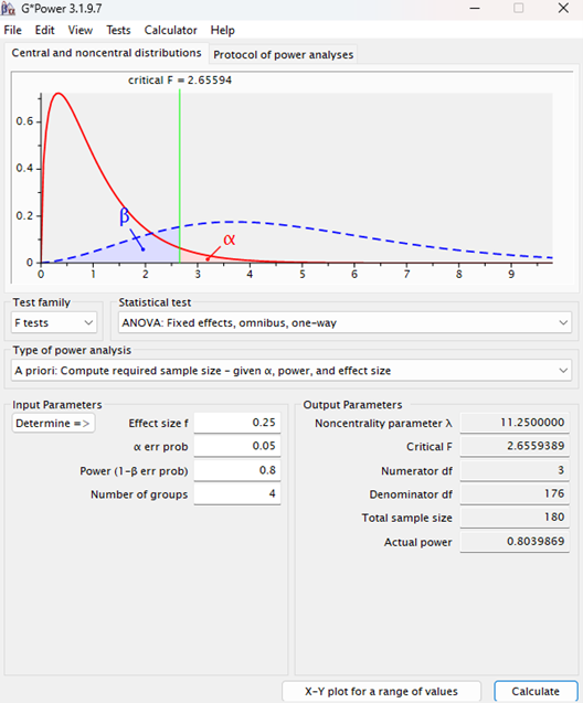
Procedure: After a power analysis using G*Power (see below), N= 180 participants are randomly assigned to receive one of the three types of preparedness messages, or no message. After reading the message, participants complete the questionnaire assessing their intentions to engage in preparedness behaviours. A one-way ANOVA is used to compare the mean preparedness intentions across the three messaging conditions.
Here is the (simulated) data from this study design:
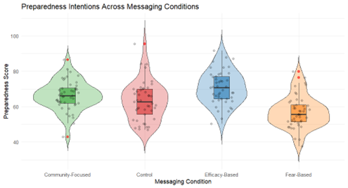
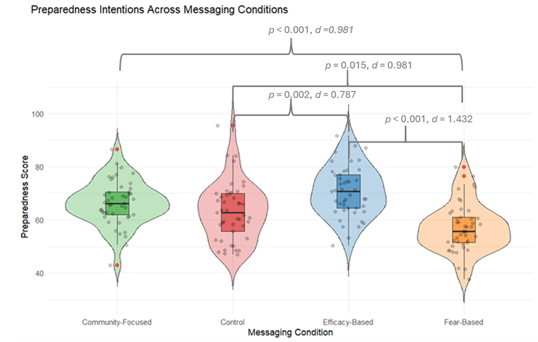
The graph shows preparedness intentions across four messaging conditions: Community-Focused, Control, Efficacy-Based, and Fear-Based (N=45 per condition). Violin plots display the distribution of scores, with wider sections indicating more frequent scores. Boxplots within the violins show the median and interquartile range, highlighting the central 50% of scores. Jittered grey dots represent individual scores, and red dots mark outliers. Efficacy-Based messaging shows the highest median and range, followed by Community-Focused, while Fear-Based, and Control conditions show lower scores.
This lecture chunk explains the above design:
8.2 The Omnibus Test
The ANOVA omnibus test is our first step in determining whether there are significant differences between our four groups.
The key idea behind the omnibus test is to assess whether at least one group mean differs significantly from the others. In our study, the ANOVA omnibus test evaluates whether the mean preparedness scores differ across the four messaging conditions. However, it does not specify which groups are different; it only tells us if a significant difference exists somewhere among the groups. If the omnibus test is significant, post hoc tests are then used to pinpoint where those differences lie.
ANOVA calculates an F-statistic by comparing two sources of variability in the data: 1. the variance between the group means (between-group variance) and 2. the variance within each group (within-group variance). As with the t-test, it’s possible to work out the F-statistic by hand, but for this course we’ll be using a stats program (JASP/SPSS/R) to perform all of this for us (see blue box below for why I don’t make you do this by hand).
8.2.1 Basic maths behind the ANOVA omnibus test
Between-Group Variance - This measures the variability of the group means around the overall mean of all groups combined. It captures how much the different messaging conditions (e.g., Efficacy-Based vs. Fear-Based) affect preparedness intentions. A larger between-group variance indicates that the group means are spread far apart, suggesting a potential effect of the messaging type.
Within-Group Variance - This measures the variability within each group around its own group mean. It reflects individual differences in preparedness intentions that are not explained by the messaging condition. High within-group variance suggests that participants' scores vary widely within each messaging condition.
Calculation of the F-statistic - The F-ratio is calculated by dividing the between-group variance by the degrees of freedom between and dividing the within-group variance by the degrees of freedom within and then dividing the products of each of those. Mathematically, this is represented as:
Let’s generate the F-statistics for the above experiment.
The following formula is used to calculate the between-group variance. In simple terms it tells us to take each group’s mean and compared them to the overall mean (grand mean) of all participants. The difference between each group mean and the overall mean is taken and then squared, weighted by the number of participants in that group (45 in all conditions), and then summed across all groups.
\[ SSB = \sum_{i=1}^{k} n_i \left(\bar{X}_i - \bar{X}_{\text{overall}}\right)^2 \]
Where:
\(n_i\) is the number of participants in group \(i\).
\(\bar{X}_i\) is the mean of group \(i\).
\(\bar{X}_{\text{overall}}\) is the overall mean of all participants.
For our data we get the following:
 Next, we need to calculate the within-group variance using the formular below.
Within each group, each participant’s score is compared to the group’s mean. The difference is squared, and these squared differences are summed for each group and then combined across all groups.
\[ SSW = \sum_{i=1}^{k} \sum_{j=1}^{n_i} \left( X_{ij} - \bar{X}_i \right)^2 \]
Where:
\(X_{ij}\) is the score of participant \(j\) in group \(i\).
\(\bar{X}_i\) is the mean of group \(i\).
\(n_i\) is the number of participants in group \(i\).
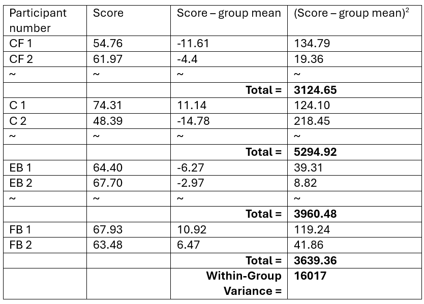
So, in other words, for this part I need to find the difference for each participant to the groups mean, square and sum that difference for each group, and then sum the group totals. Here is a snippet of how this works for the first two participants of each group, but in not going to do this by hand for all 180 participants (I do have life some of the time!), so I did the totals with code in R instead.
 The final step is to take our Between-group variance and divide that by our degrees of freedom between (number of groups – 1 = 3). And divide our within-groups variance by our degrees of freedom within (number of participants – number of groups = 176)
Between groups value = 4468/ 3 = 1489.3
Within groups value = 16017 /176 = 91.01
And then divide the between groups value by the within groups value
F ratio = 1489.3 / 91.01 = 16.36
8.3 Interpreting the results of an ANOVA omnibus test
In our study, if the F-ratio is significantly greater than 1 (which it is, F = 16.365), it suggests that the differences between the messaging conditions are larger than would be expected by chance. A significant F-value (p<0.05, which ours again is, p<0.001) indicates that at least one messaging condition has a different effect on preparedness intentions compared to the others.
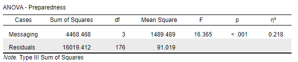
note: Number in this table differ slightly to my by hand calculation due to my rounding of numbers each step.
8.4 Post-Hoc Testing
While a significant omnibus result tells us that there is a significant difference somewhere among the group means, it does not specify where the differences lie. To identify which groups differ from each other, we need to perform additional “post-hoc” tests, to make comparisons between each individual group. In a way this turns it back into a number of 2 group comparisons, so it's tempting to just resort back to running a number of t-tests again. That’s almost what we do, but just running t-test after t-test would cause an issue with our Type I error rate.
8.5 Why we can’t just run multiple t-tests
As you likely remember from the previous chapter, when conducting statistical tests, such as t-tests or correlations, each test is associated with a specific error rate, typically set at an alpha level of 0.05. This means that for any single test, there is a 5% chance of making a Type I error (falsely rejecting the null hypothesis). This error rate is known as the “test-wise error rate.” However, when performing multiple tests on the same dataset, the probability of making at least one Type I error increases with each additional test. For instance, if you perform 20 comparisons, the likelihood is high* that at least one of the results will be statistically significant by chance alone, even if the null hypothesis is true. This accumulation of error across multiple tests is known as the multiple comparisons problem.
An ANOVA is therefore split into two separate tests. The omnibus test, a test that determines significant difference across all levels of the independent variable, and the post-hoc test, a test that looks at the difference between each individual level of the independent variable controlling for the multiple comparisons.
So, I got distracted and took a bit of a tangent when I wrote this section. Probability is hard and counterintuitive, I originally wanted to give the actual probability of a type 1 error if a study is run 20 times. But I didn’t want you to get bogged down in the value here (as that’s not the main take away) so I’ve relegated the maths to another nerdy blue box.
Question: If there is a 5% probability of a false positive in a study and we run the study 20 times what is the probability that one or more study results will be a false positive?
Probability of false positive: p=0.05
Probability of not a false positive: 1 – p = 0.95
N = 20
Probability of no false positives: P(x=0)
P(x=0) = (20 | 0)x (0.05)^0 x (0.95)^20
P(x=0) = 0.95^20 = 0.3585
Probability of more than one false positive: P(x=1)
P(x=1) = 1 - P(x=0)
= 1- 0.358 = 0.6415
This gives us a 64.15% probability that at least one out of 20 studies would produce a false positive result. To say it another way, if we ran our study 20 times and found a significant result, at some point across those 20 studies, it would be more likely than not to be a false positive. i.e. not good science!
8.6 Interpretation of post-hoc comparisons
Once again, your statistics program does the heavy statistical lifting of accounting for multiple tests and should give you a table something like this.
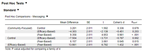
In this table you can see that each group is paired with each other group, if the p-value is less than 0.05 we can say that there is a difference between those two groups. This can take a bit of effort to get your head around in table form, so here is the graph again, this time with the significant differences added.
8.6.1 Test yourself
Look back at the hypotheses from earlier. Are all of them confirmed? See if you can explain the results in real world terms, what have we actually found? Which technique(s) do you suggest we use and why?
This lecture chunk explains the above analysis:
In the next chapter we'll work through the analysis for different types of one-way ANOVA