4 Assumption checks of t-tests and other difference tests
4.1 Why We Run Assumption Checks for T-Tests
Before conducting a t-test, it's essential to check that the data meets specific assumptions required for the test to produce valid and reliable results. The primary reason for running these assumption checks is that t-tests rely on certain mathematical properties, such as the normality of data and equal variances between groups, to accurately determine whether differences between group means are statistically significant. If these assumptions are violated, the t-test may yield misleading results, increasing the risk of Type I or Type II errors (see section on statistical power for more detail on type errors).
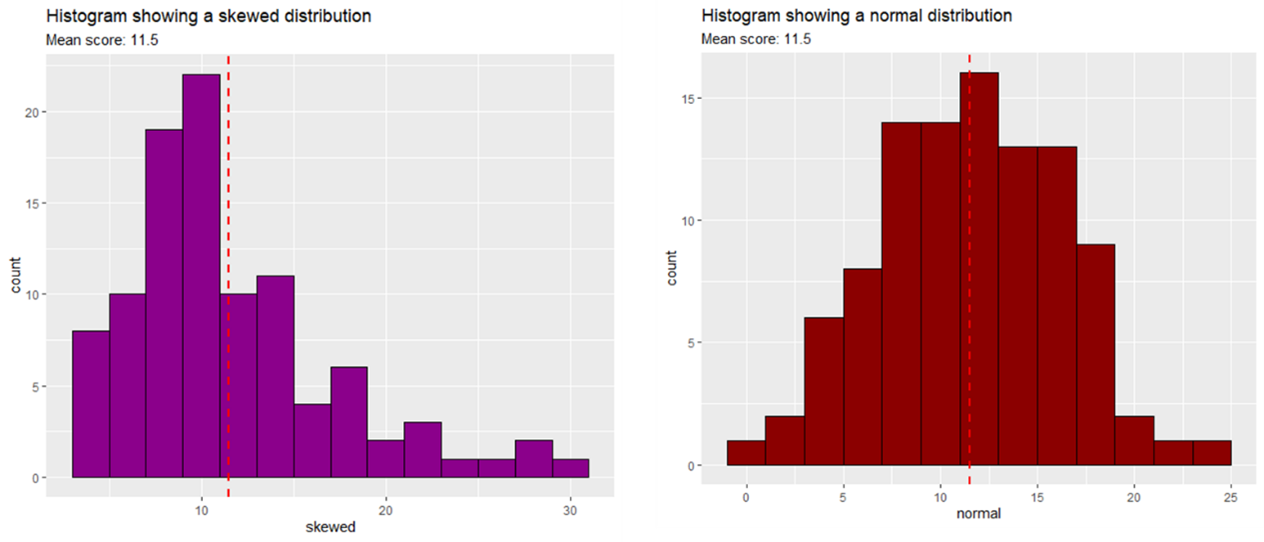
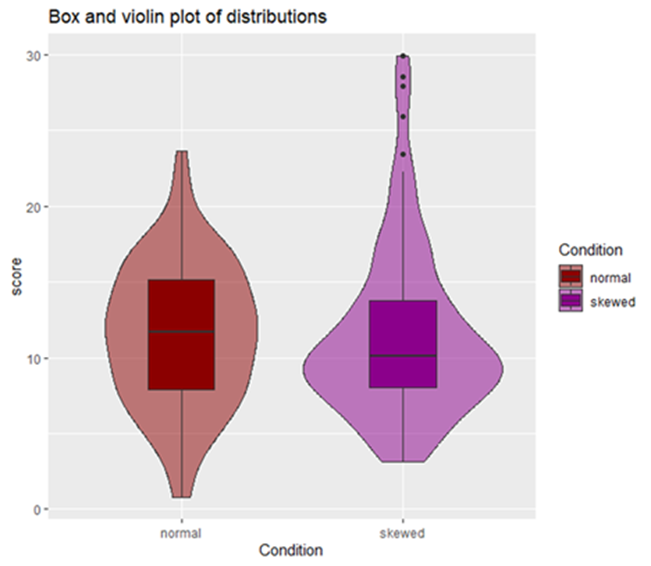
To illustrate why assumptions are critical, consider that t-tests use the mean as the measure of central tendency. However, if your data is not normally distributed or if the variance between groups is unequal, the mean may not accurately represent the central tendency of your data (see the below histograms with the same mean but different levels of normality). This could lead to incorrect conclusions about the differences between groups.
The following video is an extract from one of my lectures where I explain the concept of assumption checks for t-tests
4.2 Assumption 1: Type of Data
T-tests are designed for use with interval or ratio data, where the differences between values are meaningful and consistent across the scale. These types of data allow for precise measurement of differences in means between groups. In contrast, ordinal data, which ranks data without assuming equal intervals between ranks, is not suitable for t-tests because the test assumes that the dependent variable is measured on a continuous scale.
Using ordinal data in a t-test can lead to inaccurate results because the distances between data points are not consistent or quantifiable in the same way they are with interval or ratio data. For example, if you were to rank participants' satisfaction levels from 1 to 5, the difference between a 1 and a 2 might not be the same as the difference between a 4 and a 5, making the mean a less reliable measure of central tendency.
4.3 Assumption 2: Normal Distribution
One of the critical assumptions of the t-test is that the dependent variable is normally distributed within each group. Normality is essential because the t-test relies on the distribution of the sample means to be approximately normal, especially when sample sizes are small. This assumption allows the test to accurately assess whether the observed difference between group means could have occurred by chance.
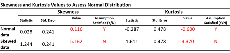
To check for normality, you can use visual methods like histograms or Q-Q plots, or statistical tests such as the Shapiro-Wilk test (see JASP example for how to read such a test). If your sample size is large (typically over 50 observations per group), visual inspection of histograms or using the skewness and kurtosis statistics may suffice. For smaller samples, the Shapiro-Wilk test is recommended. If the test indicates a significant deviation from normality, the assumption is violated, and you may need to consider a non-parametric alternative.
For Small Samples (n < 50): Calculate the skewness or kurtosis value and divide it by its standard error. If the resulting value falls within the range of -1.96 to 1.96, the data is likely normal.
For Larger Samples (50 < n < 300): Use a wider range of -3.29 to 3.29 for the skewness or kurtosis value divided by its standard error to assess normality.
If the skewness and kurtosis values fall within their respective ranges, your data likely meets the normality assumption. If they fall outside these ranges, you may need to consider transforming the data or using a non-parametric test instead.
The below table shows the values for the two variables presented in the figure above.
4.4 Assumption 3: Homogeneity of Variance
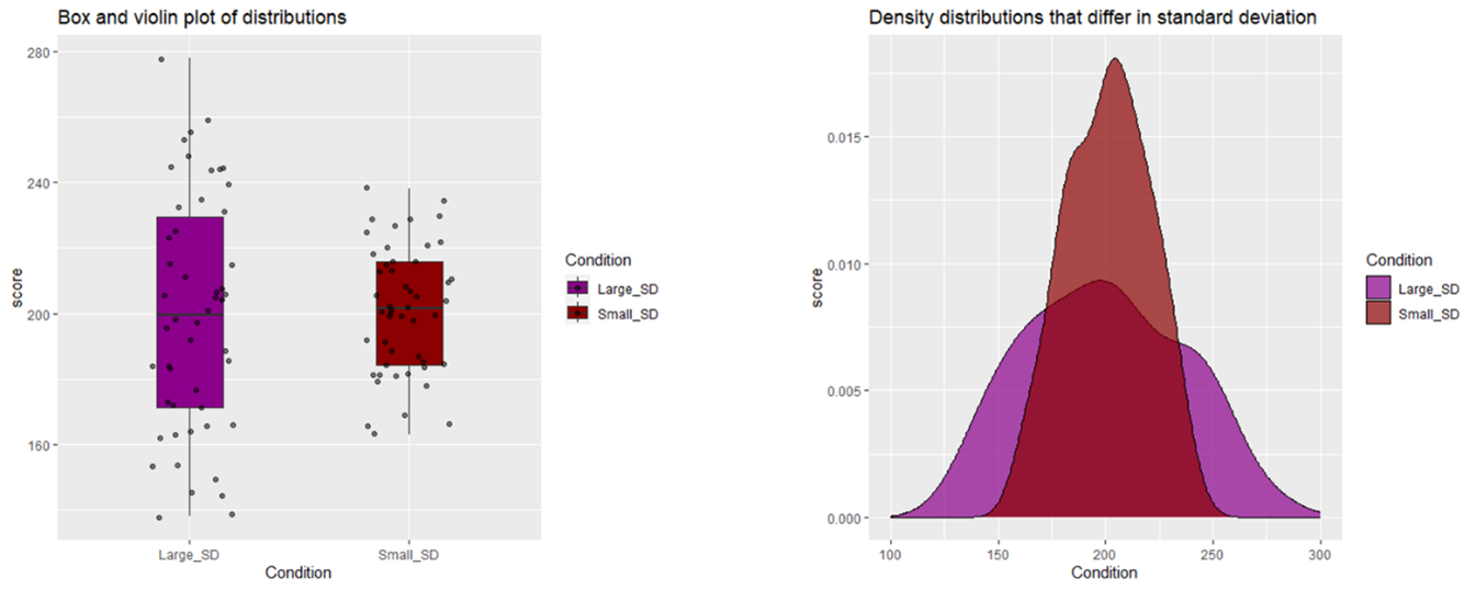
The assumption of homogeneity of variance states that the variance (the square root of standard deviation) within each of the groups being compared should be roughly equal. This assumption is crucial for the t-test because it ensures that the groups are comparable, allowing the test to accurately assess differences in means.
The below images illustrate a violation of the assumption of homogeneity of variance. They demonstrate how the purple variable has a much larger variance than the red variable, however, they are both still normally distributed.
To statistically test for homogeneity of variance, you can use Levene’s test, which compares the variances of the groups. If Levene’s test is significant, it indicates that the variances are not equal, and the assumption of homogeneity of variance is violated. In such cases, you might need to consider an alternative non-parametric test.
In the next chapter we will work through two examples of t-test analysis using data and worksheets that you can find on Moodle.