10 Factorial ANOVA (Important for your assignment)

In the previous chapter, we explored one-way ANOVA, a statistical method used to compare means across three or more groups when you have a single independent variable. But sometimes we want to fit more than one independent variables into our research. This is where factorial ANOVA comes into play.

Factorial ANOVA allows us to examine the effects of multiple independent variables on a dependent variable, as well as the interactions between these factors. In this chapter, we'll work through the basics of factorial ANOVA using a 2x2 (pronounced two-by-two) design as an example. We'll explore how to interpret main effects and interaction effects, and understand how these contribute to our overall understanding of the data.

10.1 What is a Factorial ANOVA?

A factorial ANOVA is an extension of the one-way ANOVA that includes two or more independent variables. Each independent variable, or factor, can have multiple levels. When combined, these factors create various conditions or groups. The "factorial" aspect refers to the fact that every level of one factor is combined with every level of the other factors.

For example, in a 2x2 factorial design, there are two independent variables, each with two levels, resulting in four unique experimental conditions.

The following lecture chunk introduces you to the concept of factorial ANOVA:

10.2 Example of a factorial ANOVA design

Let's consider a study designed to investigate how the presentation of climate change information across different psychological distances affects changes in risk perception. This experiment employs a 2x2 between-subjects factorial design, manipulating temporal distance (now vs. future) and physical distance (near vs. far). The dependent variable is the change in risk perception, measured as the difference between pre- and post-presentation scores.

Research Question: How do temporal and physical distances in the framing of climate change information influence changes in risk perception?

Design: A 2x2 between-subjects factorial design.

Independent Variables:

1. Temporal Distance (Between-Subjects)

   • Now: Information presented as an immediate threat.

   • Future: Information presented as a distant future threat.

2. Physical Distance (Between-Subjects)

   • Near: Information framed as affecting a geographically close location (e.g., within the participant’s country).

   • Far: Information framed as affecting a geographically distant location (e.g., another continent).

Dependent Variable:

• Change in Risk Perception: Calculated as the difference between post-presentation and pre-presentation risk perception scores. Higher values indicate a greater increase in perceived risk.

Hypotheses

H1: Temporal distance will have a main effect on the change in risk perception, with information presented as a near-term threat (now) resulting in a greater increase in risk perception compared to information presented as a future threat.

H2: Physical distance will have a main effect on the change in risk perception, with information presented as affecting a near location resulting in a greater increase in risk perception compared to information presented as affecting a far location.

H3: There will be a significant interaction between temporal and physical distance on the change in risk perception, with the combined effect of near-term and near-location presentations leading to the greatest increase in risk perception.

Procedure

1. Participant Recruitment: Recruit N = 128 participants (as specified by an a-priori power analysis) who are randomly assigned to one of the four conditions, ensuring equal group sizes (n = 32 per condition).
2. Pre-Presentation Measure: All participants complete a baseline measure of risk perception using a standardised risk perception scale.
3. Presentation of Information:

• Now, Near Condition: Immediate threat affecting a nearby location.
• Now, Far Condition: Immediate threat affecting a distant location.
• Future, Near Condition: Future threat affecting a nearby location.
• Future, Far Condition: Future threat affecting a distant location.

4. Post-Presentation Measure: After the presentation, participants complete the risk perception scale again.
5. Calculation of Change Scores: The change in risk perception is calculated by subtracting pre-presentation scores from post-presentation scores.

10.3 Visualizing Factorial ANOVA Data

With a four-condition setup, it's tempting to visualise the data as we did for the one-way ANOVA—treating each combination of factors as its own separate condition. This approach allows us to compare across the four conditions to see where the differences lie.

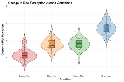
And from this, we can already start to see differences between the conditions. However, this method somewhat misses the core aspect of our study design. We have two separate independent variables, each with two levels, and this factorial structure isn't well presented in the previous image. By visualising the data this way, we treat each combination as an isolated condition, neglecting the interactions between the variables.

To better capture the relationships in our data, it makes more sense to use a line graph with 95% confidence intervals. This type of visualisation reflects both the main effects and the interaction effect between the two variables. It allows us to see how the effect of one independent variable may depend on the level of the other independent variable. Here is the same data presented as a line graph:

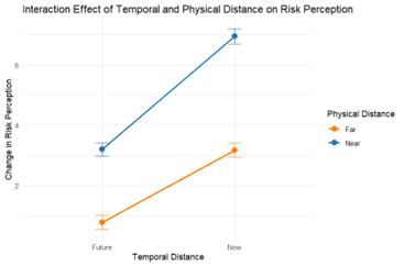
From the line graph we can now see that risk perception increases when climate change is presented as an immediate threat ("Now") compared to a future threat ("Future"), this is the main effect of Temporal Distance. Additionally, risk perception is higher when the threat is framed as affecting a nearby location ("Near") rather than a distant one ("Far"), this is the main effect of Physical Distance.

Importantly, the lines are not parallel, suggesting a significant interaction effect between Temporal and Physical Distance. Specifically, the combination of presenting climate change as both immediate and nearby results in the greatest increase in perceived risk, while the effect is less pronounced when either the temporal or physical aspect is framed as distant.

But as always, we need to check to see if these differences are occurring by chance or if it is likely to be the experimental manipulation that is causing these differences. For that we need to return to statistical analysis.

The following lecture chunk is me further explaining this design:

10.4 Conducting a Factorial ANOVA

10.4.1 The Omnibus Test

In factorial ANOVA, the omnibus test is our first step in assessing whether there are any statistically significant effects within the data. This test evaluates the main effects of each independent variable as well as any interaction effects between them. The main effects tell us whether each independent variable (e.g., Temporal Distance and Physical Distance) independently influences the dependent variable. The interaction effect, on the other hand, tests whether the impact of one independent variable depends on the level of the other variable. Importantly, the omnibus test does not specify which groups are significantly different from one another; it simply tells us if there is a statistically significant effect present in the data, either in the main effects or in the interaction.

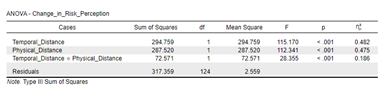
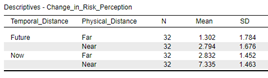
In this example we can see that we have a significant main effect for both temporal distance and physical distance, and a significant interaction effect. We can look at the descriptive statistics to determine the direction of each of the main effects.

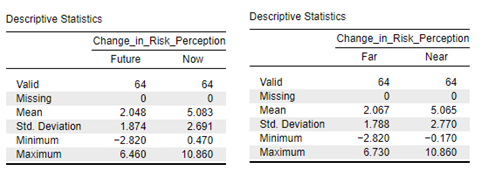
The mean dependent variable value (which is the difference in risk perception before and after the presented information) for the “Now” information framing is significantly higher than that of the “Future” information framing and the mean dependent variable value for the “Near” information framing is significantly higher than the “Far” information framing.

The interaction effect, however, takes a little more thought.

10.4.2 Interaction Effect

The interaction effect shows whether the effect of one independent variable on the dependent variable changes depending on the level of the other independent variable. In our study, for instance, the interaction effect reveals that the impact of Temporal Distance on risk perception varies depending on whether the information is framed as "Near" or "Far." This is crucial because it highlights the combined influence of both factors, providing a deeper understanding than looking at the main effects alone. If an interaction effect is significant, it suggests that the factors do not operate independently of each other but rather interact in a way that influences the outcome variable.

It’s possible to determine this from the breakdowns of means.

However, it is far easier to determine this from the line graph, see pervious section.

10.4.3 Post-Hoc Tests in Factorial ANOVA

Once the omnibus test reveals significant effects, particularly interaction effects, post-hoc tests are needed to pinpoint exactly where these differences lie. Post-hoc tests in factorial ANOVA are used to explore the specific group comparisons that are driving the significant findings observed in the interaction or main effects. These tests make pairwise comparisons between the levels of the independent variables while controlling for the increased risk of Type I errors that comes with multiple testing. For example, if the interaction effect is significant, post-hoc tests will help determine whether the difference between “Now” and “Future” is significant at both levels of Physical Distance (“Near” and “Far”), and vice versa. Essentially, post-hoc tests break down the overall effects detected by the omnibus test into specific, interpretable comparisons, allowing for a more detailed understanding of the nature of the effects in the data.

10.4.4 Assumption checks

Before interpreting the results of a factorial ANOVA, it is crucial to ensure that the data meet the necessary assumptions for this type of analysis. These assumptions are similar to those discussed in the chapter on t-tests, specifically the assumptions of homogeneity of variance and normality. However, there are some key differences in how these assumptions apply when conducting a factorial ANOVA.

Homogeneity of Variance, refers to the assumption that the variance within each group (or condition) is equal. In a factorial ANOVA, this assumption must be met not just across the levels of a single independent variable (as in a one-way ANOVA or independent samples t-test), but across all combinations of levels for both (or more) independent variables. For example, if we have a 2x2 design with Temporal Distance and Physical Distance as independent variables, we must ensure that the variance in each of the four unique conditions (e.g., "Now_Near", "Now_Far", "Future_Near", "Future_Far") is similar. Violations of this assumption can lead to biased F-statistics, making it difficult to trust the results of the ANOVA. The Levene’s Test is typically used to check this assumption, and in a factorial ANOVA, it assesses variance across all conditions simultaneously.

Normality refers to the assumption that the dependent variable is normally distributed within each group. In factorial designs, we must ensure that normality holds within each combination of the independent variables. While minor deviations from normality are unlikely to impact results significantly, severe violations can lead to incorrect inferences. As with the t-test, this assumption can be evaluated using visual inspections of histograms or statistical tests like the Shapiro-Wilk test. In factorial ANOVA, however, the complexity increases with each additional independent variable, as normality must be checked within each subgroup.

Factorial ANOVA also assumes that the observations are independent of each other, just as in simpler designs. This means that there should be no systematic relationship between the scores of participants in different conditions. While this assumption may not require statistical testing, it should be ensured during the design and data collection phases.