16 Multiple regression

Multiple regression is a method that helps us predict an outcome variable based on several independent variables. It is a technique that tells us which variables are the most important for predicting an outcome, and how such predictor variables interact. By building a prediction model, multiple regression allows us to understand how variables are connected and helps us make powerful data-informed decisions.

16.1 Shared variance with multiple variables

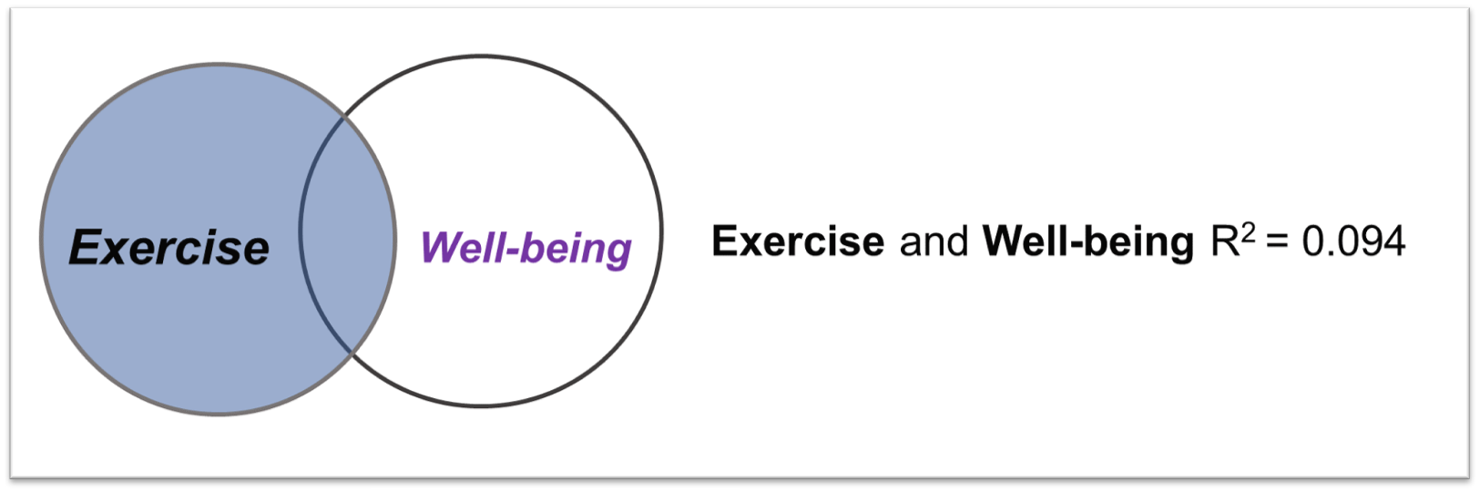
In the previous chapter on simple linear regression, we suggested that one predictor variable (exercise) shared variance with another variable (well-being). Visually, this can be represented using a Venn diagram with two circles: one for exercise and one for well-being. The overlap between these two circles represents the shared variance, or the extent to which variations in exercise can explain variations in well-being. This shared variance can be represented numerically as the square of the correlation coefficient between the two variables. In this hypothetical example exercise is correlated with well-being with a correlation coefficient of r=0.307 (i.e. a moderate-positive correlation) and, as such, it can be said that exercise explains 9.4% of the variance in well-being (\(R^2\)=0.094)

In a multiple regression analysis, we use two or more independent variables to predict the value of a dependent variable. In doing so, each independent variable may share some variance with the dependent variable, but also shares variance among the other independent variables. Understanding this shared variance is crucial for interpreting the results of a multiple regression analysis.

For instance, let's say we're using three independent variables to predict well-being: exercise, age, and income. Each of these variables could contribute to the variance of well-being.

When we add the variables one-by-one, the overlap of each independent variable circle with the well-being circle represents the unique shared variance each variable contributes to well-being.

When adding our samples age data, to help us explain well-being, we see significant correlations for the three different relationships. 1. a positive correlation exists between exercise and well-being, 2. a negative correlations exist between age and well-being 3. a negative correlation between age and exercise.

Because the \(R^2\) is derived from squaring an r value, and when you square any negative value, it loses its negative sign.

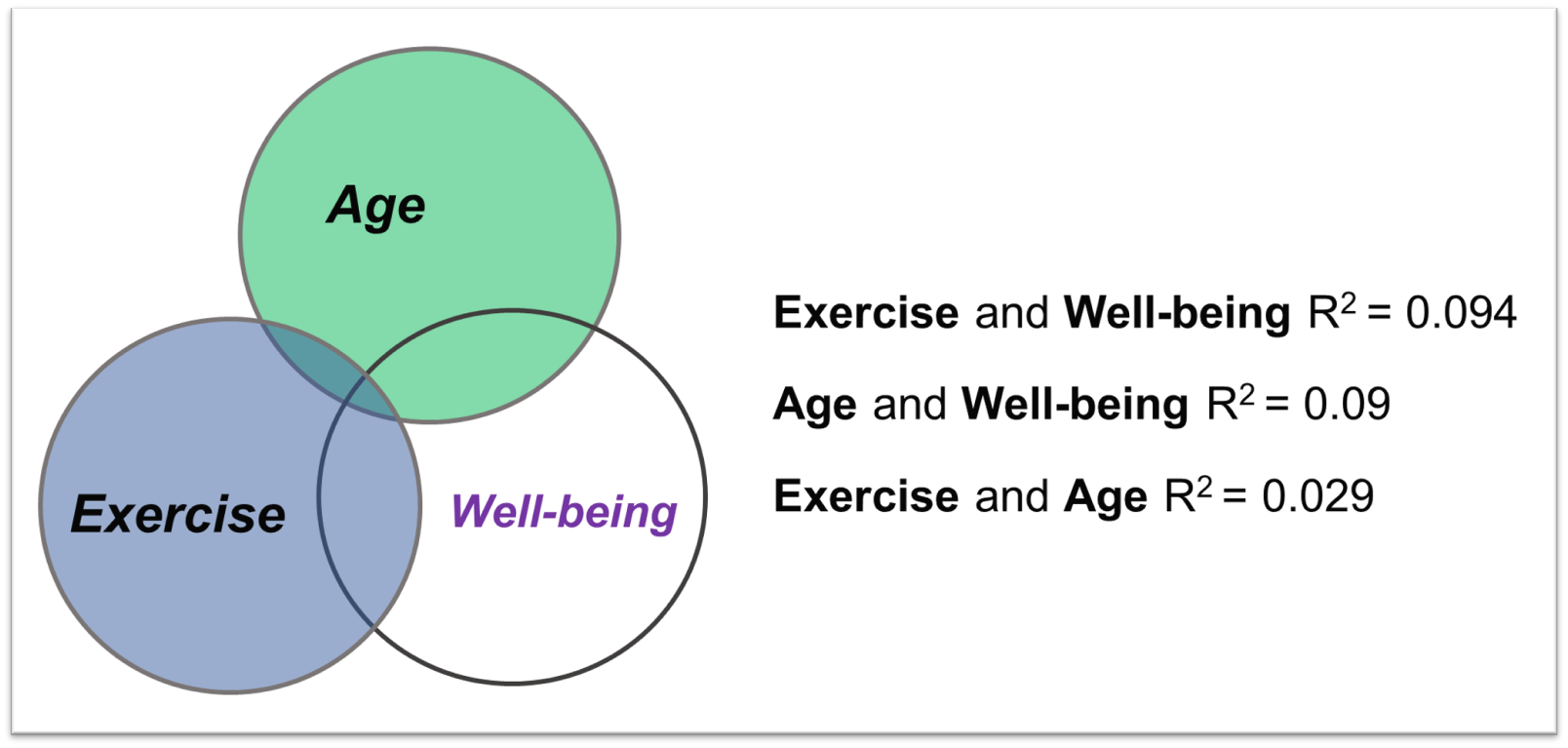
Both age and exercise now explain some of the variability in well-being, and since they are also related to each other, some of the variance they explain overlaps.

Finally, when we add income, we find that the variable shares variance with both age and well-being. Income therefore adds more variance explained to our model while also overlapping with some of the variance explained by age

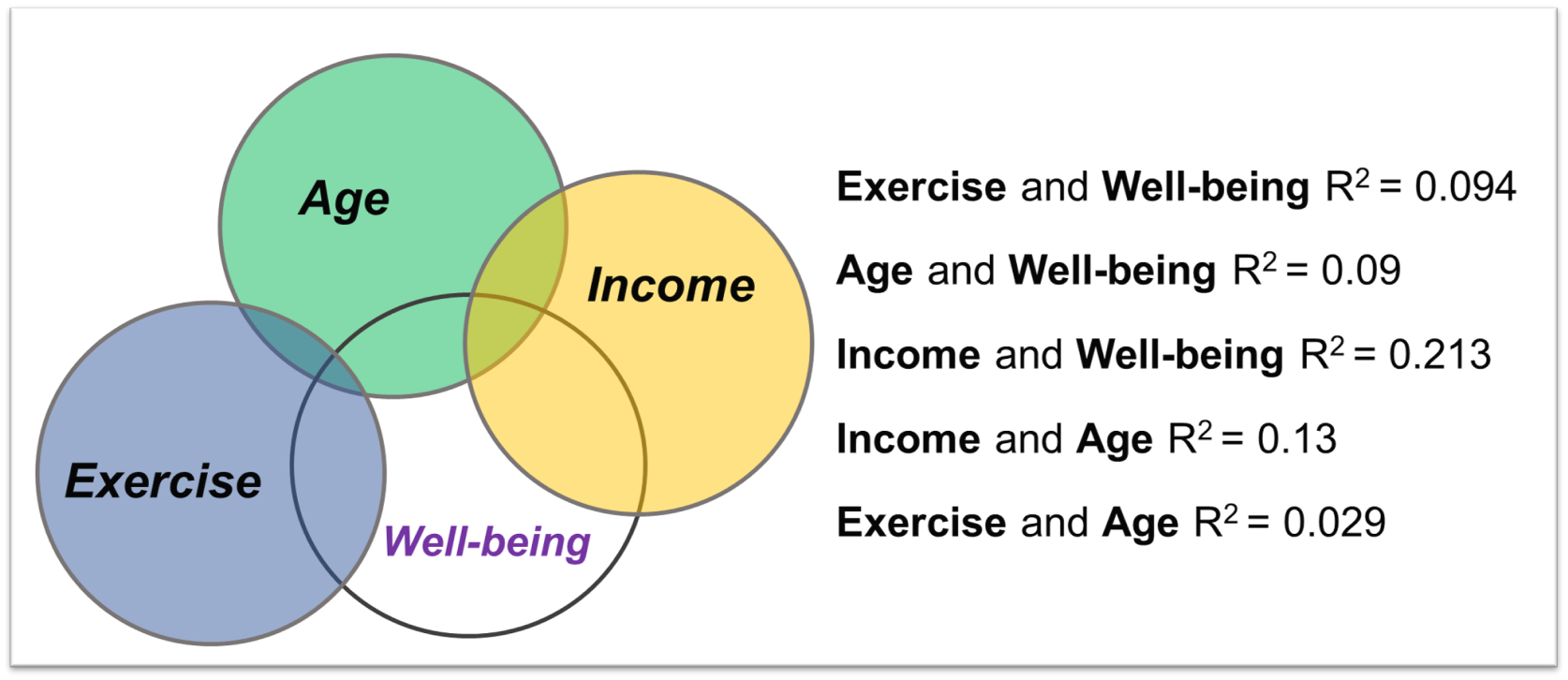
The outcome of this is that each variable that we add here allowed us to better explain our concept of well-being. And as such, if we were to know a person's amount of exercise, age, and income we could predict their well-being to a greater degree than if we just know their amount of exercise.

It's important to understand that the Venn diagrams in this guide offer a simplified representation of variance explained by predictor variables in a regression model. In reality, when two predictor variables have overlapping variance, this shared variance can contribute more to the model than what the individual variables might suggest. This occurs due to interaction effects, where the combined influence of two predictors can explain more variance in the dependent variable than the sum of their individual effects. When looking at the Venn diagrams, remember that this additional explained variance from interactions isn't explicitly depicted, but it's crucial to consider when interpreting regression results.

This is why, as you'll see later on, the final \(R^2\) is greater than the sum of all the simple (univariate) regressions.

16.2 The Regression Equation

As you've probably realised, using Venn diagrams to illustrate the relationships among multiple variables can get quite confusing, especially when there are numerous variables that all have some degree of correlation with each other. That's where the regression equation comes in handy.

The regression equation is a mathematical representation of the relationships among the variables in a multiple regression analysis. It shows how the dependent variable is predicted by the independent variables. In its abstract form, the regression equation can be written as:

\[ y = \beta_0 + \beta_1x_1 + \beta_2x_2 + \ldots + \beta_kx_k + \varepsilon \]

Here, \(y\) is the dependent variable, \(x_1\), \(x_2\),...,\(x_k\) are the independent variables (i.e. the amount of exercise, age, and income of the participants), \(\beta_0\) is the intercept, \(\beta_1\), \(\beta_2\),...,\(\beta_k\) are the coefficients for the independent variables, and \(\varepsilon\) is the error term, representing the unexplained variability in the dependent variable (i.e. the left over white space in the Venn diagram figure above).

The intercept \(\beta_0\) represents the value of the dependent variable when all independent variables are zero. This \(\beta_0\) is equivalent to the intercept, \(c\), value in the equation from last week.

The coefficients (all the remaining \(\beta\) values) represent the average change in the dependent variable for a one-unit change in the respective independent variable, holding all other variables constant. Just like the gradient of the line \(m\) value in the equation from last week. The "..." and the \(k\)'s are just a way of saying "add in as many beta values as you have variables in your model".

Running our regression analysis allowed us to substituent numbers for all of the coefficients to the degree that all we are left with are \(x\)'s, that we can use to sub in our data.

16.3 Interpreting a regression model

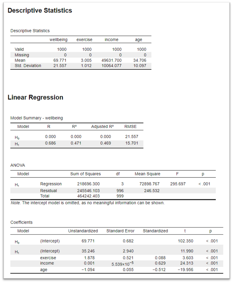
I will explain the steps for running a regression model, in full, in this weeks JASP workshop. For now, I want us just to focus on the interpretation. Here is the JASP output for a model that uses the variables exercise, age and income to predict well-being scores.

Let's break this down by table.

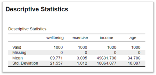
16.3.1 Descriptive statistics

The descriptive statistics are useful for context. This detail isn't given here but I can tell you that in this dataset (N=1000), the well-being score is out of 100, the exercise variable is based off of number of hours of exercise a week, income is in £GBP, and age is in years.

16.3.2 Model Summary

The Model Summary table provides an overview of the overall performance of the regression model. It contains key statistics that helps us assess how well the model fits the data.

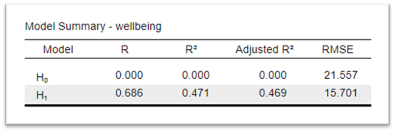
The table contains two rows \(H_0\) and \(H_1\). \(H_0\) refers to the null model, a model that assumes that none of the predictors in the model have an effect on the dependent variable, meaning that the coefficients for all predictors are equal to zero. \(H_1\) is our alternative model, the model containing our variables. This is the line that interests us.

The main details of interest are:

• The Adjusted \(R^2\) Value: This is a modified version of \(R^2\) that takes into account the number of independent variables in the model. It allows us to say how much variance in our dependent variable is explained by our predictor variables.

• RMSE: RMSE stands for Root Mean Square Error. It is a measure of the differences between values predicted by a model and the values actually observed. RMSE is a measure of how spread out the residuals are. In other words, it tells you how concentrated the data is around the line of best fit. It is used as our \(\varepsilon\) in the regression model.

We will often take the Adjusted \(R^2\) for multiple regression and the \(R^2\) only for simple regression (regression with just one predictor variable). For our well-being model, the Adjusted \(R^2\) of 0.469 tells us that our three variables together explain 46.9% of the variability in well-being. Which is pretty good.

16.3.3 ANOVA

The ANOVA table provides information about the overall significance of the model. It shows whether the model is better at predicting the dependent variable than a model with no independent variables (i.e., the null model).

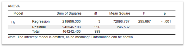
The findings from this table will need to be reported in our write-up, however, to interpret it, all we actually need is the p-value. A significant finding on this test tells us that our model is significantly better than the null model.

ANOVA stands for ANalysis Of VAriance. We'll come back to ANOVA in week 4. For now, just think of it as a slightly fancier t-test, a test that compares across groups (rather than correlates). In this case it is comparing the null model to the alternative model and seeing if they are significantly different.

16.3.4 Coefficients

Finally, to understand the role of each variable in the model we need to look at the coefficients table.

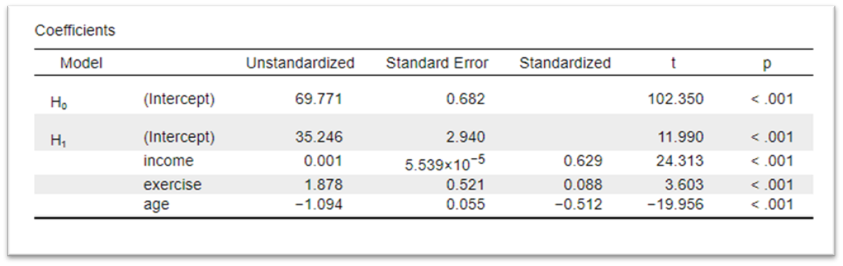
This table provides detailed information about the individual variables in the model. It includes statistics for each independent variable and the intercept for the model.

There are two columns that are key to our understanding of the model. The Unstandardized column and the p column.

Starting with the p column, this is the probability of obtaining a t-value as extreme as the one observed if the null hypothesis is true. A small p-value indicates that the variable plays a statistically significant role in our model. It could be the case that we include a variable that is not related to our dependent variable or the variance it explains is accounted for by other variables in the model. In those cases, the p-value would be above 0.05. A p-value of <.001 for all three of our variables indicates that they are all relevant to include in our model.

The values in our Unstandardized column correspond to the \(\beta\) values in our regression equation. They play the same role as the gradient of the line of best fit from simple regression last week. They represent the absolute change in the dependent variable for a one-unit change in the independent variable, holding all other variables constant.

In our model, this table tells us that:

1. For every 1 hour increase of exercise a week, well-being increases by 1.88 points.
2. For every 1 year of ageing, well-being decreases by 1.09 points.
3. For every £1 of income, well-being increased by 0.001 points.

That last finding is not as intuitive as it could be, so it makes sense to convert income into values of 1000's of pounds (i.e. if someone earns £32500 a year they can be said to earn 32.5 thousand pounds a year). To do this all I need to do is divide each of our income values by 1000 and run the model again.

Doing so gives us this:

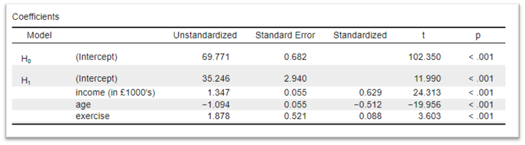
3. For every £1000 of income, well-being increases by 1.35 points.

16.4 Building our regression equation from the model

From this we can now start building out our regression equation. We have three variables predicting well-being so all we need to do is fill in the \(\beta\) values and the \(\varepsilon\) in the following equation.

\[ Wellbeing = \beta_0 + \beta_1income + \beta_2age + \beta_3exercise + \varepsilon \]

\(\beta_0\) = The unstandardized (beta) value for the intercept of \(H_1\) = 35.25

\(\beta_1\) - \(\beta_3\) = the unstandardized (beta) value of the three variables = 1.35, -1.09 and 1.88

\(\varepsilon\) = the Root Mean Square Error (RMSE) of \(H_1\) = 15.7

This give us the following regression equation:

\[ Wellbeing = 35.25 + 1.35income -1.09age + 1.88exercise + 15.7\]

From this equation, if we knew an individual's income, age and how much exercise they engaged in per week we could estimate their well-being with a fairly high degree of accuracy.

Alongside the equation it is important to note our Adjusted \(R^2\) of 0.469, and indicate that this means that over half of the variability in well-being is not explained by the variables we have included in the model.

16.5 So what?

What is the point of doing all this work? Well, if I'm wanting to increase the well-being of my local community this finding might put me off putting money into community exercise classes. While there all likely other benefits of such an intervention, there are only so many hours in a week and, based on this data, a 1.88 point increase in well-being (on a scale out of 100) for an extra hour of exercise might not be the most cost-effective way of spending my limited pool of money.

Then again, it's not like we can stop someone from ageing, or increase their income. Perhaps further research that compares the effects of, for example, exercise, mindfulness and diet, while controlling for demographic factors, would be useful to inform what type of intervention might be more cost-effective.

16.6 Week 2 - Test yourself mcq’s

1. What is multiple regression?
   Using a single categorical variable to predict the value of a dependent variable.A method that helps predict an outcome variable based on one independent variable.A method that helps predict an outcome variable based on several independent variables.A measure of the association between two variables.
2. What is the regression equation?
   A graphical representation of the relationships among the variables.A mathematical calculation of the shared variance.A mathematical representation of the relationships among the variables in a multiple regression analysis.An empirical observation of the relationships among the variables.
3. In the regression equation, what do the β values represent?
   The dependent variable.The coefficients for the independent variables.The error term.The independent variables.
4. What do the values in the Unstandardized column in the coefficients table represent?
   the shared variance between the variables.the average change in the dependent variable for a one-unit change in the respective independent variable, holding all other variables constant.the correlation coefficient between the variables.the absolute value of the correlation coefficient between the variables.
5. What does the Adjusted \(R^2\) value tell us in a multiple regression analysis?
   The strength of the linear relationship between the dependent variable and each independent variable.The shared variance among the independent variables.The percentage of variability in the dependent variable that is explained by the predictor variables.The effect size of the independent variables on the dependent variable.