17 Statistical assumption checks for multiple regression
At this point in your studies, it's important for you to understand how to assess and report the statistical assumptions underlying regression analysis. However, it's not until more advanced stages in your career that you'll learn how to address such violations of assumptions.
For now, just interpret and report these assumptions. If the results deviate greatly from the assumptions, then it's important to report such deviations and state that findings "should be taken with caution".
Here are the key assumptions in multiple regression and how to check for them:
17.1 Check for Linearity
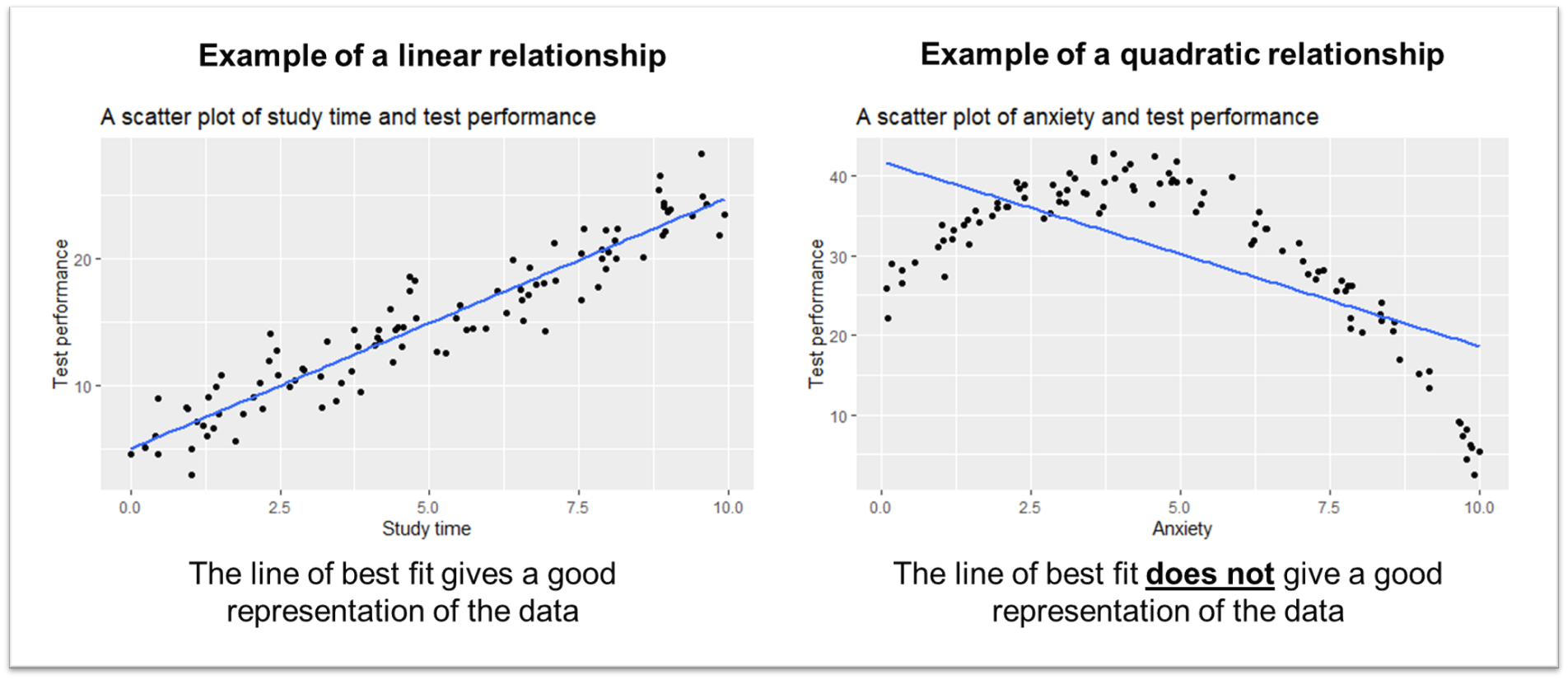
The assumption of linearity states that the relationship between the independent and dependent variables is linear. You can check this visually by examining scatter plots of the independent variables against the dependent variable.
17.2 Check for Multicollinearity
Multicollinearity occurs when two or more independent variables in a regression model are closely related, making it difficult to disentangle their individual effects on the dependent variable. This can lead to unstable coefficient estimates, as small changes in the data can result in significant changes in the estimates. You can assess multicollinearity by creating a correlation matrix of the independent variables and looking for variables with a correlation coefficient greater than 0.7 or less than -0.7. However, this is not a strict rule, just an indication of a strong correlation.

In the table above, suppose we use these five personality constructs to predict a behaviour, such as recidivism. Checking the correlation coefficients, the largest value is -0.368, indicating that multicollinearity is not likely an issue in this case. Be mindful not to confuse correlation coefficients with p-values, as it's an easy mistake to make.
While multicollinearity can make interpretation challenging, it's not necessarily a deal-breaker. In some cases, the focus may be on predicting the outcome rather than interpreting the individual contributions of each predictor. For a more in-depth discussion on multicollinearity and its implications see Vatcheva et al (2016).
17.3 Check for Outliers
Outliers are data points that differ significantly from other observations. They can be detected through various methods. In a boxplot, outliers are typically displayed as individual points outside the whiskers, which extend from the first and third quartiles (Q1 and Q3) to Q1 - 1.5 * IQR (interquartile range) and Q3 + 1.5 * IQR, respectively (see this link for a full explanation of how read a boxplot).
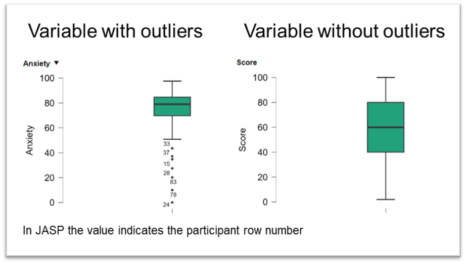
JASP can automatically identify outliers in boxplots, making it easier to spot them. However, addressing outliers is often a contentious issue because their treatment can have a significant impact on the results of a statistical analysis. The decision to keep or remove outliers depends on multiple factors.
First, it's important to consider the context of your data. Outliers could be the result of measurement errors, data entry errors, or other random anomalies. However, they could also represent genuine extreme values that offer valuable insights. For example, in a study on wealth distribution, billionaires would be outliers but they are a real-world phenomenon that might be important to the research.
Secondly, outliers can heavily influence other data assumptions, such as linearity, normality of residuals, and homoscedasticity. It is crucial to evaluate whether outliers are affecting these assumptions and to justify their removal or retention. This, in fact, can be a way of addressing the violations of assumptions listed in this chapter.
Thirdly, outliers can disproportionately affect key statistical measures like the mean and standard deviation. It's very easy to fall into the trap of removing outliers until a significant results appears. This kind of practice may fall into that grey area of academic misconduct that we discussed in first year, known as Questionable Research Practices.
Ultimately, the decision to handle outliers involves a balance of statistical judgment and domain expertise. It's necessary to ensure that any decision involves transparently reporting and justifying your decisions.
17.4 Checks of residuals
The last two assumption checks require an examination of the residual. Residuals are a fundamental concept in regression analysis, representing the difference between observed and predicted values of the dependent variable. In a simple regression, we visualised the predicted value with our line of best fit, and the observed values are just the data points in our relationship.
For each observation, a residual is calculated by subtracting the predicted value from the observed value. In simple linear regression, where there is one independent variable, the residual for each observation is the distance from the data point to the regression line. In multiple regression, it is the distance from the observation to the regression plane.
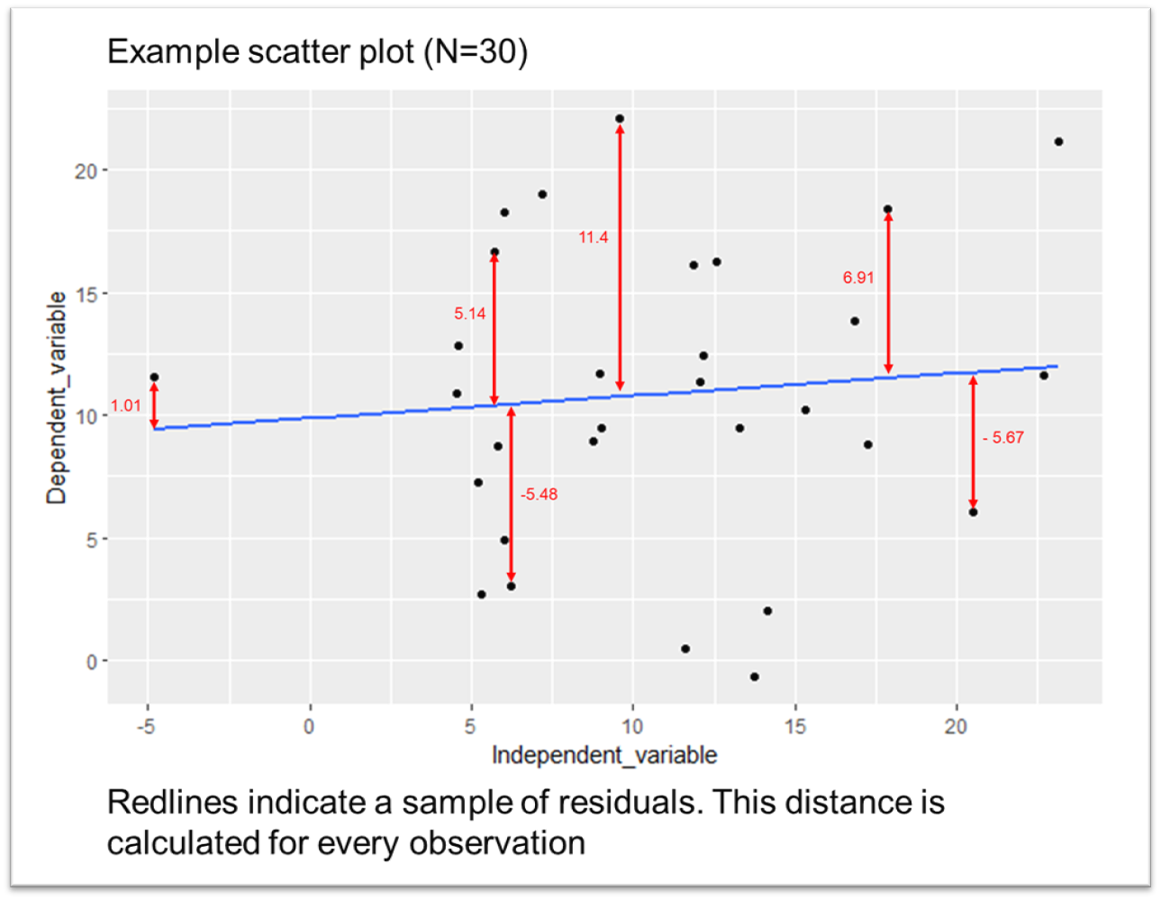
The goal of regression analysis is to minimize the residuals, or in other words, to make the predicted values as close as possible to the observed values. Residuals can be used to evaluate the fit of a regression model, to detect outliers, and to check for any violations of the assumptions of regression.
17.4.1 Check for Normality of Residuals
The assumption of normality of residuals is important for hypothesis testing in linear regression. It ensures that the standard errors of the coefficients are unbiased and that the significant testing for the coefficients are valid. This, in turn, helps us make valid inferences about the relationships between the variables.
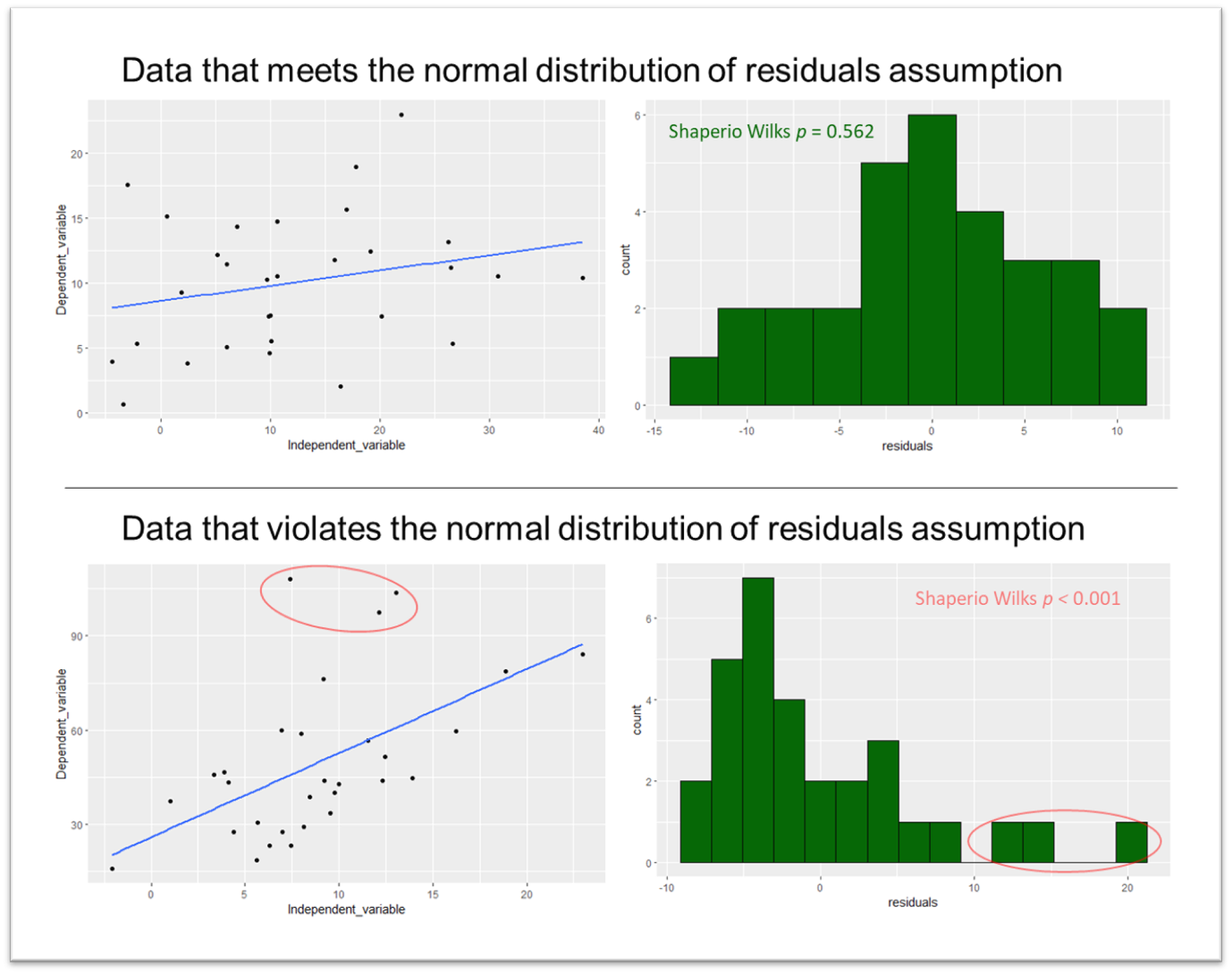
In contrast, checking for normality of the individual variables is not required for linear regression. Instead, the focus is on the distribution of the residuals, which should be normally distributed if the model's assumptions are met. The residuals represent the differences between the observed and predicted values of the dependent variable, and their distribution tells us about the model's fit and the relationships between the variables.
If you're working on a program where you can calculate the residuals, then you can check the normality of the residuals using the Shapiro–Wilk test or by assessing the skewness and kurtosis. In JASP the only means of checking the normality of residuals is through the normality of residuals plot option.
17.4.2 Check for Homoscedasticity
Homoscedasticity, the word that strikes fear into undergrad (and most postgrad) psychology students throughout the land, is not as complicated as it sounds.
"Homos": Greek for "same" or "equal." In the context of homoscedasticity, it refers to the equality or sameness of the variances.
"Skedasis": Greek word related to the concept of dispersion or spreading out. In statistics, it is associated with the variance or scatter of data points.
The scatter plots below demonstrate how such data might look. Heteroscedasticity (i.e. different "spreadness") means that the line of best fit becomes less reliable at different points in the model.
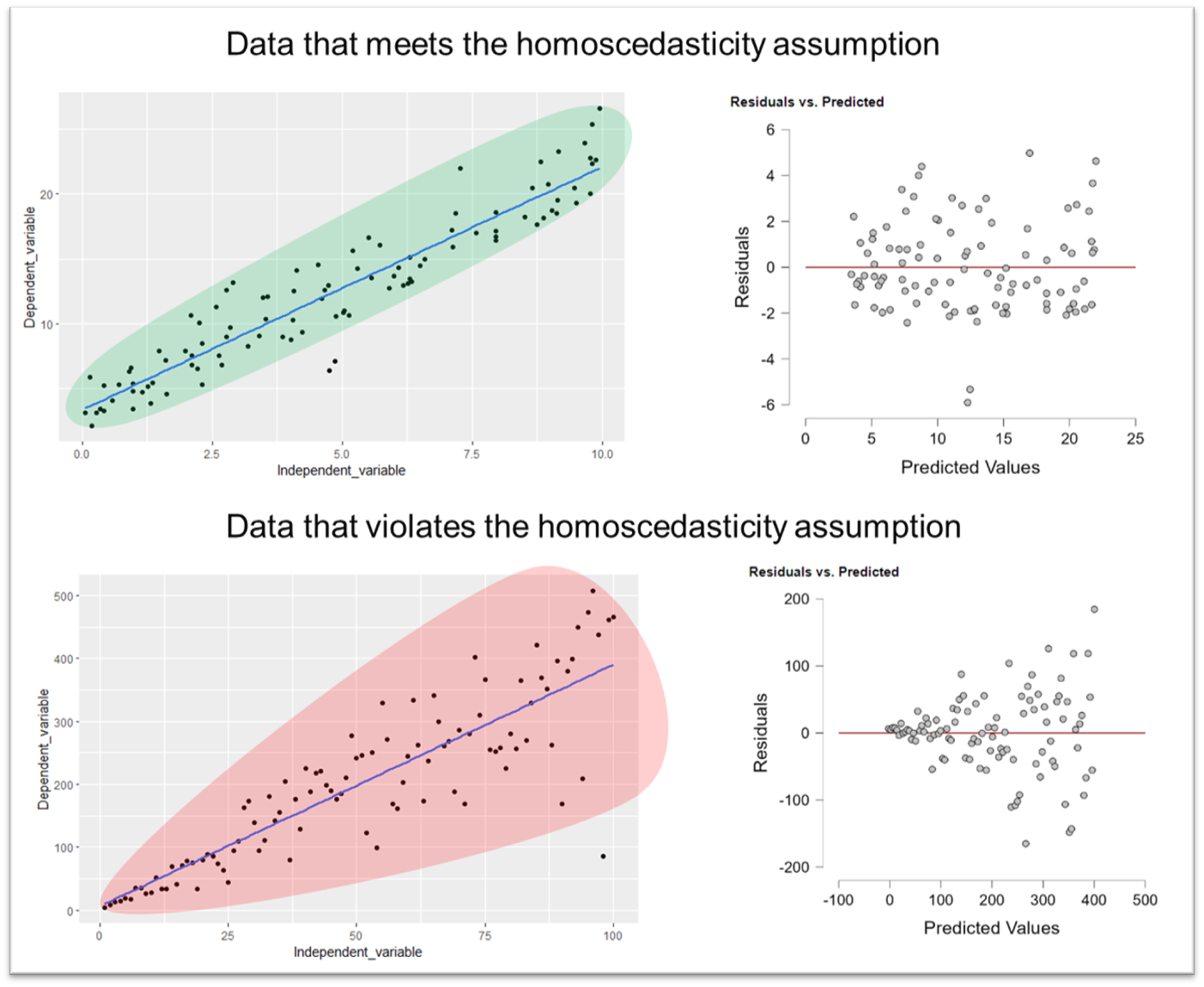
In this context, what we're looking for is an equal distribution of data points along the line of best fit, avoiding a funnel-shaped pattern. When dealing with regression analyses that involve more than two predictor variables, it's often not feasible to visualise the data. In such cases, a plot of predicted variables against residuals can be used to check for homoscedasticity. In this plot, we are, again, looking for the absence of a funnel shape in the points.
This check can also be performed using z-scores of the predicted values against the residuals; a level line in this context would indicate homoscedasticity (a uniform spread of the residuals). This method is used in software like SPSS for checking homoscedasticity, so you may see some other guides talking about this if you read wider on the topic.