7  Session 4

8 Statistical modeling in R

8.1 Session overview

In this session we’re finally going to get to statistical analysis!

In your undergraduate course this is likely where you would start, with a pristine dataset, all setup with neat variable ready to go. Hopefully you can see from the past few weeks how uncommon this actually is in real world research.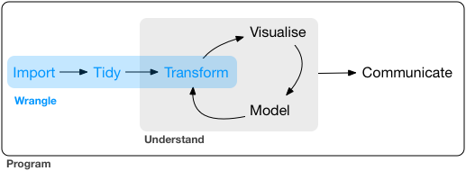

We are now at the visualise, model and communicate stage of this diagram.

In this session we will run through two forms of regression analysis that you’ll be choosing from for your assignment: Multiple (linear) Regression and Binary Logistic Regression.

Hopefully you’ve already attended the NS7151 sessions on the statistical theory related to this material. If not, I recommend taking a look at my undergraduate handbook, chapters 13-19, here:https://richclarkepsy.github.io/NS5108/introduction-to-regression-analysis.html

When working in R, the process of regression analysis has two steps:

1. Run the model, which you can then interpret.

2. Check whether the model meets its statistical assumptions.

Note, this is actually the opposite order to the way you will report your results. However, you can only check the statistical assumptions once you have a fitted model (due to the need to examine the module residuals). When it comes to interpretation and reporting, you should always start with the assumption checks. Only if the assumptions are reasonably met, should you move on to interpreting the results.

8.2 Multiple Regression

We’ll start with multiple (linear) regression. This is where we predict a continuous outcome (for example: WEMWBS wellbeing score) from several predictors (in this case: age, BMI, physical activity, rural/urban).

The workflow in R looks like this:

1. Set your working directory, load your packages and read in the data.

2. Wrangle the data ready to create the model

3. Fit the regression model with the lm() function.

4. Use the fitted model object to check assumptions.

5. If assumptions are reasonably met → read and interpret results.

6. Present the results in an APA style table.

Key assumptions for multiple regression:

• Linearity: Each predictor has a linear relationship with the outcome. Checked with scatterplots.

• No multicollinearity: Predictors shouldn’t be strongly correlated. Checked with correlations and/or Variance Inflation Factor (VIF).

• Normality of residuals: The model errors(AKA residuals) should be normally distributed. Checked with a histogram and the Shapiro Wiks test.

• Homoscedasticity: Equal spread of residuals across predicted values. Checked with scatter plot of predicted values against residuals, and a statistical test.

8.2.1 Step 1 - Read in a wrangle the data

As with all session, restart, get a fresh script, set your working directory, and read in your data.

Then create a dataset with just the WEMWBS wellbeing score, age, BMI, physical activity, and rural/urban. I’ve given you the code in the chunk below. This is a combination of the code you’ll have learnt in sessions 1 & 2 of this course.

Code

# intended model WEMWBS ~ age, bmi, physical activity, rural/urban 

library(tidyverse)

shes_2022_data <- read_csv("SHeS_2022_clean.csv")

shes_m_regression <- shes_2022_data %>%
  mutate(wemwbs_score = wemwbs_optimistic + wemwbs_useful + 
           wemwbs_relaxed + wemwbs_interested_in_people + 
           wemwbs_energy + wemwbs_dealing_problems +
           wemwbs_thinking_clearly + wemwbs_good_about_self + 
           wemwbs_close_to_others + wemwbs_confident + 
           wemwbs_make_up_mind + wemwbs_loved + 
           wemwbs_interested_in_new_things + wemwbs_cheerful,
         bmi = weight_kg_self_adj / ((height_cm_self_adj / 100) ^ 2)) %>%
  select(id, wemwbs_score, age, bmi, urban_rural, mvpa_mins_week_10min_bouts)

8.2.2 Step 2 - Create the model

Next, to run our multiple regression we need to use the lm() function. Within the function we will need to point to our dataset that contains the cleaned variables and indication how we’d like the model to be organised. We’ll need to assign the output of the function to an object which we will later turn into a readable format.

The following code creates our model:

Code

wemwbs_model <- lm(wemwbs_score ~ bmi + age + mvpa_mins_week_10min_bouts + urban_rural,
                   data = shes_m_regression)

When writing the lm() expression you may have noticed that you do not get the auto-complete for your variable names. This is partly due to us not piping in the data, so the expression only knows the dataset at the end of the expression, but also something to do with the way the expression parses the data.

The important aspect for you is to make sure you double check you have the exact variable names that you want to use in your anlysis, otherwise you’ll hit an error

8.2.3 Step 3 - Check regression assumptions

There are a number of ways we could check the statistical assumptions for our analysis. For the purposes of this course I suggest extracting the residuals and predicted/fitted values from the model and then create figures using the ggplot() function that we covered in the last session. We can also apply statistical tests to that data that we extract.

Residuals are the differences between the values your model predicts and the values you actually observe. In other words, each residual shows how far off the model was for that specific data point.

Checking residuals matters because most of the key assumptions in linear regression are about the pattern of those differences. If the residuals look roughly normally distributed, have constant spread across the range of fitted values, and don’t show obvious patterns, then the model is more likely to be giving trustworthy estimates, tests and confidence intervals. If the residuals show strong patterns, skew, or changing variance, it suggests the model may not fit well and that the results could be misleading.

I explain more in this section of my undergraduate materials: https://richclarkepsy.github.io/NS5108/statistical-assumption-checks-for-multiple-regression.html#checks-of-residuals

Code

shes_m_regression_assumptions <- shes_m_regression %>%
  drop_na() %>%
  mutate(model_residuals = wemwbs_model$residuals,
         model_fitted = wemwbs_model$fitted.values)

8.2.3.1 Normality of residuals

The following code uses the ggplot() function from last week to create a histogram of the residuals of the model. For us to meet the statistical assumption for linear regression this histogram needs show a normal distibution.

Code

shes_m_regression_assumptions %>%
  ggplot(aes(x=model_residuals)) +
  geom_histogram(fill = "darkblue", colour = "black") +
  labs(title = "Histogram of residuals") +
  theme_light()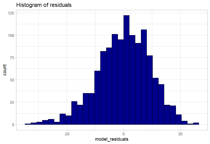

Do we meet this statistical assumption?

Well, it’s a judgement and an argument that we can make. We have a slight left-skew, but in my opinion looks minor.

We can collect some further evidence for us to judge by runnign a statistical test. The Shapiro Wilk test takes our distribution and compares it to a perfect normal distribution. If it is significantly different then that implies that we have non-normal data (in this case our model residuals).

The following code runs that test:

Code

shapiro.test(shes_m_regression_assumptions$model_residuals)

The “e” is scientific notation. It means “× 10 to the power of…”. So:

9.137e-07 = 9.137 × 10⁻⁷, which is just a very small number written in a shorter form.

In ordinary decimal form it would be:

0.0000009137.

If you want to get R to show you the number with all its 0’s you can select that as an option at the start of your code. But be warned it, it can sometimes lead to hard to read outputs if the number is very small (or large)

Code

options(scipen = 999)

shapiro.test(shes_m_regression_assumptions$model_residuals)

The test is SignificantNon-significant

Therefore we have metviolated our statistical assumption of normality of residuals.

This is sometimes the issues with large datasets, and in fact its suggested that Shapiro Wilk only be used for samples of around a maximum of 50. So lets take this with a pinch of salt. Ideally we should manually do a skewness and kurtosis check. Explained here if you’d like to give it a go.

8.2.3.2 Homoscedasticity and heteroscedasticity

Homoscedasticity means the residuals have constant spread across all levels of the predicted values. In other words, the “amount of error” is roughly the same everywhere.

Heteroscedasticity means the residuals have changing spread — the errors get larger or smaller in a pattern (for example, a funnel shape). This breaks a key assumption of linear regression and can make tests and confidence intervals unreliable.

A plot of the residuals vs fitted values can check this concept.

Code

shes_m_regression_assumptions %>%
  ggplot(aes(x = model_fitted, y = model_residuals)) +
  geom_point() +
  geom_hline(yintercept = 0, colour = "red") +
  labs(x = "Fitted values", y = "Residuals",
       title = "Residuals vs Fitted plot") +
  theme_minimal()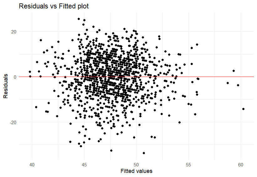

Here’s how it works, simply:

If the points are evenly scattered around the horizontal line (as in the plot here), it suggests homoscedasticity, the variance of the errors is constant.

If the points fan out, narrow in, or form a clear pattern, that suggests heteroscedasticity.

From this plot I feel confident in making the argument that we have met the homoscedasticity statistical assumption.

We can add further evidence to this by running an additional test in this case a Non-Constant Variance test, which is interpreted in the same way as Shapiro Wilk.

Code

# this test requires the "car" package. install and load before use

ncvTest(wemwbs_model)

If so read the # comment, install the car package, load the package and try again.

If not, will done for reading the comment and following the instruction.

The test is SignificantNon-significant

Therefore we have metviolated our statistical assumption of normality of homoscedasticity.

8.2.4 Step 4 - Interperting the model

Now that we have the checks out of the way we can go ahead and intrepret the model.

r’s built in function to do this is summary(), and not summaries() which my fingers always seem to want to type first.

Code

summary(wemwbs_model)

For our model this gives us an output in the console that looks something like this.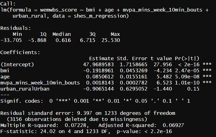

Here’s a breakdown of what you see here:

1. The model that was called. the code from earlier to run our model. To the left of the ~ is our dependent variable to the right are all the variables in our model

2. Some statistics around the residuals that I never use, but could loosely be used to judge the assumption checks.

3. The coefficients (variables) in the model. Estimate indicating the degree to which the Dependent Variable increases for each increment of increase in the predictor variable. The intercept value in this column is used to write your regression equation,

4. Std. error, a measure of certainty for each of the variables

5. t and p values, used to indicate if the variable is significant in the model. * indicate levels of significant.

6. The end text allows us interpret if the model as a whole is significant and the adjusted R-squared. This indicates the percentage of variance of the DV explained by our model variables.

This is a little messy for my liking so lets turn this into something more readabel. For this you will need to install the sjPlot package. Note the capital P.

Code

library(sjPlot)

tab_model(wemwbs_model)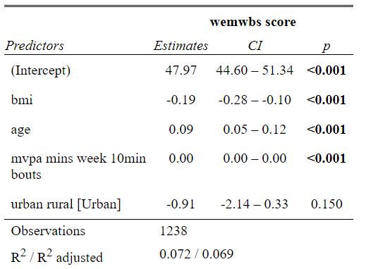

Nice! But we can even tidy this up a bit more:

Code

tab_model(wemwbs_model,
  title = "Multiple regression predicting WEMWBS wellbeing score",
  dv.labels = "WEMWBS score",
  string.pred = "Variables",
  show.std = TRUE,
  show.ci = FALSE,
  show.stat = TRUE,
  digits = 3,
  pred.labels = c("(Intercept)",
                  "Body Mass Index (BMI)",
                  "Age (years)",
                  "MVPA (minutes per week, 10-min bouts)",
                  "Urban vs Rural"))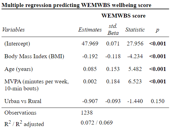

If you click the show in new window button. This will open as a html object. for here you can save and open it in word as an edited version if you want to make any tweaks for your report.

8.3 Logistic regression

Logistic regression requires a few more steps, but to make things equivalent for the assignment we’ll focus less on the assumption checks.

For this example let’s look at predicting a hypertension diagnosis with the variables of BMI, the Scottish Indices of Multiple Deprivation, income (in quintiles), and smoking status.

8.3.1 Step 1 - wrangle the data for a logistic regression.

Select out the variables of interest and perform any data transformations that are needed.

In this example we’ll calculate BMI as a continuous variable and use it as such. However, we could use BMI in its categorical from for this analysis if we so wished.

Code

hypertention_data <- shes_2022_data %>%
  mutate(bmi = weight_kg_self_adj / ((height_cm_self_adj / 100) ^ 2)) %>%
  select(hypertension, bmi, simd20_quintile, income_quintile_oecd, current_smoker) %>%
  drop_na()

An additional step we need, is to tell the program that there is an order to some of our variables. Right now when we look at the structure (str()) of our dataset our variables are character (chr) or number (num) variables. The number variables are fine for use however the character variables need to be linked to an order(i.e. most deprived to least deprived for our SIMD variable).

To do this we need to change the variable from character to a factor. This is a special variable that links each response to an order that we set.

Code

hypertention_data <- hypertention_data %>%
  mutate(hypertension = factor(hypertension, 
                               levels = c("No", 
                                          "Yes")),
         simd20_quintile = factor(simd20_quintile,
                                  levels = c("Most deprived (Q1)", 
                                             "Q2", 
                                             "Q3", 
                                             "Q4", 
                                             "least deprived (Q5)")),
         income_quintile_oecd = factor(income_quintile_oecd,
                                       levels = c("Lowest (Q1)", 
                                                  "Q2", 
                                                  "Q3", 
                                                  "Q4", 
                                                  "Highest (Q5)")),
         current_smoker = factor(current_smoker,
                                 levels = c("Never smoked or used to smoke cigarettes occasionally", 
                                            "Used to smoke cigarettes regularly", 
                                            "Current cigarette smoker")))

To find the labels for other variables dont forget you can always run the following code to get these easiely. Its worth copy and pasting from the output as these will need to be exact or the mutate will not work.

Code

hypertention_data %>%
  group_by(income_quintile_oecd) %>%
  summarise(n = n())

8.3.2 Run the logistic regression model

As with the multiple regression this code to run a logistic regression is fairly short. However it will only run if the data is first set up correctly.

Code

hypertention_model <- glm(hypertension ~ bmi + simd20_quintile + income_quintile_oecd + current_smoker, 
                          data = hypertention_data, 
                          family = binomial)

8.3.3 Assumption check

At this stage the only assumption check that I expect to see is the VIF statistic, this will give you a sense of multicollinearity. Interpretation of this statistic can be found here.

to run the check you will need the car package loaded.

Code

vif(hypertention_model)

8.3.4 Reading and interpreting the model

Code

summary(hypertention_model)

sjPlot::tab_model(hypertention_model)

plot_model(
  hypertention_model,
  show.values = TRUE,
  value.offset = .3,
  title = "Adjusted Odds Ratios for Hypertension")

What I’m thinking with this analysis is that it might make more sense to use the least deprived and the highest income as the comparison groups. We can go back to stage one and do that.

8.4 That’s all you need to know!

That’s it you now have all of the code needed to run the analysis for your assignment.

Here are the steps in full:

1. Open a new R script
2. Save the script to your working directory (wherever you store the data)
3. Set your working directory
4. Choose the variables for your analysis
5. Wrangle your data so your varibles are ready to go
6. Run your chosen model
7. (for multiple regression) visualise your residuals and interpret if you’ve meet the statistical assumptions.
8. Interpret your model findings
9. Create an appropriate table
10. (for logistic regression) visualise your findings.