Code
2 + 2
10 - 3
6 * 7
9 / 2
2^5          # powers
(3 + 5) * 2 # brackets control orderOkay, lets get you coding!
Firstly, R is an excellent calculator. Take the following lines of code and try running them in the console typing out each and hitting enter.
2 + 2
10 - 3
6 * 7
9 / 2
2^5 # powers
(3 + 5) * 2 # brackets control orderR shows results as vectors (ordered lists). [1] just means “this line begins at element 1”. You’ll later see [11], [21], etc., whenever long outputs wrap to a new line. In short, don’t worry about it, they can be ignored.
For the majority of this module I will be asking you to add and edit code in the script window. This is going to let us keep your code tidy and readable, meaning that your cleaning and analysis is reproducible by others and, most importantly, by you at a latter date!
In RStudio: File → New File → R Script.
Type some code, e.g.:
(65*0.1) + (38*0.9)

(68*0.1) + (45*0.9)

(75*0.1) + (72*0.9)
One of the ways to run code from a script is to use the Run button in the top-right of the script panel. However, you should try to resist using this button when at all possible.
You’ll have a smoother time with R if you keep your hands on the keyboard as much as you can. So instead:
Move the cursor with the arrow keys to the line you want to run (it can be anywhere on that line).
Press Ctrl + Enter (Windows) or Cmd + Enter (Mac).
To run several lines, hold shift select the lines you want and use the same shortcut.
Why bother, why not just click?
Keyboard-first running is faster, stops you accidentally executing huge chunks, and helps you step through your code deliberately.
Trust me, you’ll have a far better time with R if you resist using the mouse as much as possible.
To move from “R as calculator” to the next level we can assign values to what are known as objects. You can think of an object as a labelled box that holds the value of whatever you put in it.
To assign to an object you will need to use this notation <- which is the less than sign and a minus sign put together to form an arrow.
See what happens when you run the following code:
x <- 10
y <- 3
x + yHave you found the best way to copy code from this book yet?
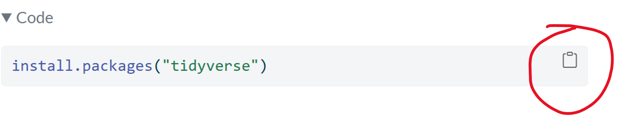
This will copy all of the text in the code box and will prevent you having to highlight it using the mouse where you can potentially miss bits. A frequent cause of errors!
Two more new terms for you now: “function” and “argument”
We call a function, that then acts on our data. Arguments go inside the brackets and give parameters for what we want the function to do.
round(3.14159, digits = 2)In the code above:
round is the function name.
3.14159 is the first argument.
digits = 2 is a named argument telling round()how man decimal places to round to.
Assign nine divided by seven to an object and then round the object to two digits.
What value do you get?
x <- 9/7
round(x, digits = 2)
Here are two more functions, run them and see if you can work out what they do:
sqrt(16)
mean(c(1, 5, 9))c() stands for combine/concatenate. It makes a vector: a single, ordered list of values. Many R functions (like mean()) expect one vector as their main input.
Here, c(1, 5, 9) creates a numeric vector containing 1, 5, and 9, and mean() averages that vector.
Why not mean(1, 5, 9)?
Because mean() expects one main argument (x). If you write mean(1, 5, 9), R treats 1 as the data, and the extra numbers as other arguments (e.g., trim, na.rm), which is not what you want and can cause warnings or errors. Always wrap multiple values with c().
Quick facts about c()
Works for any type: c(1, 2), c("a", "b"), c(TRUE, FALSE).
If you mix types, R coerces to a common type (e.g., c(1, "a") becomes character).
You can also assign c() to an object. ages <- c(12, 24, 48, 76)
If you ever want to know more about a function you can use the following notation:
?round # shows you the help page for round()Question: What does the # character do in an R script?
Across this module (and your assignment if you’re taking NS7154) you’ll work with a cleaned extract of the Scottish Health Survey (SHeS). SHeS monitors the health of people living in Scotland. It includes health conditions, risk factors, wellbeing, and inequalities. It ran in 1995, 1998 and 2003, then annually since 2008.
On Moodle you will find the .csv file of the cleaned data (SHeS_2022_clean.csv) and a word document that contains information related to each variable (Assignment dataset codebook.docx)
I’ll explain more about the dataset and your assignment in class. For now just download these files.
Just email me on rclarke8@glos.ac.uk and I’ll see if I can share it with you. It’s open access data but I needed a licence to use it for educational purposes and so I don’t host it online.
The working directory is the folder that R treats as “home” for your current session. When you read or write files without giving full paths, R looks inside this folder by default.
Often in R you are working with multiple data files, importing some and exporting others. A working directory directs Rstudio towards where you want all of this activity to happen.
Setting up a nice neat working directory is the first thing I do when starting up a new research project. And setting the working directory is the first thing you’ll need to do each time you want to work on your analysis.
Step 1
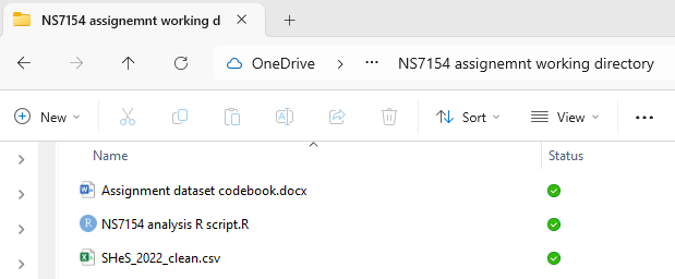
Create a folder for this module, e.g., NS7154 assignment working directory, and place your dataset and codebook in that folder.
Step 2
Create a new R script in RStudio and save that script to your working directory folder.
You should now have three files in that folder, the data, the codebook and the r script (a .R file)
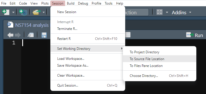
Step 3
Within RStudio click Session -> Set Working Directory -> To Source File Location
Step 4
To check that this has set your working directory successfully you can run the following code. Running the first line will show you where you are currently working from and the second line will list the files that are in your current working directory.
getwd()  # where am I? (prints the working directory)

list.files() # list files/folders in the working directory
If list.files() gives you anything other the three files mentioned earlier, go back and check steps 1 - 3 again.
Within your new analysis script, delete any of the previous code you might have on the script and add these two lines.
library(tidyverse)

shes_2022_data <- read_csv("SHeS_2022_clean.csv")If you’re typing the code and paying attention to the autocompleate you may have noticed read.csv as an additional option. The read.csv function comes from base R, while read_csv is from the readr package, part of the tidyverse. While it requires an extra step to install and load read_csv its worth it for three reasons:
Unlike read.csv, read_csv does not convert character strings into factors by default. This gives you more control over how your data is read and interpreted.
read_csv returns tibbles rather than traditional data frames. While they may seem identical, tibbles have several advantages that make them work better with the rest of the tidyverse packages. For instance, tibbles retain the data type of each column, do not convert character vectors to factors by default, and have improved printing methods.
read_csv handles missing values (NAs) in a more straightforward manner and makes data cleaning and manipulation processes easier.
Is this the dullest note in the whole book? Maybe, I at least feel it’s a strong contender.
Running these lines will load the tidyverse package and read in your data. If all is good you should see a new object in your environment window.
This is the data all set up ready for our further wrangling and analysis. To see your data you can use any of the following lines of code:
glimpse(shes_2022_data)And your RStudio should now look something like this:
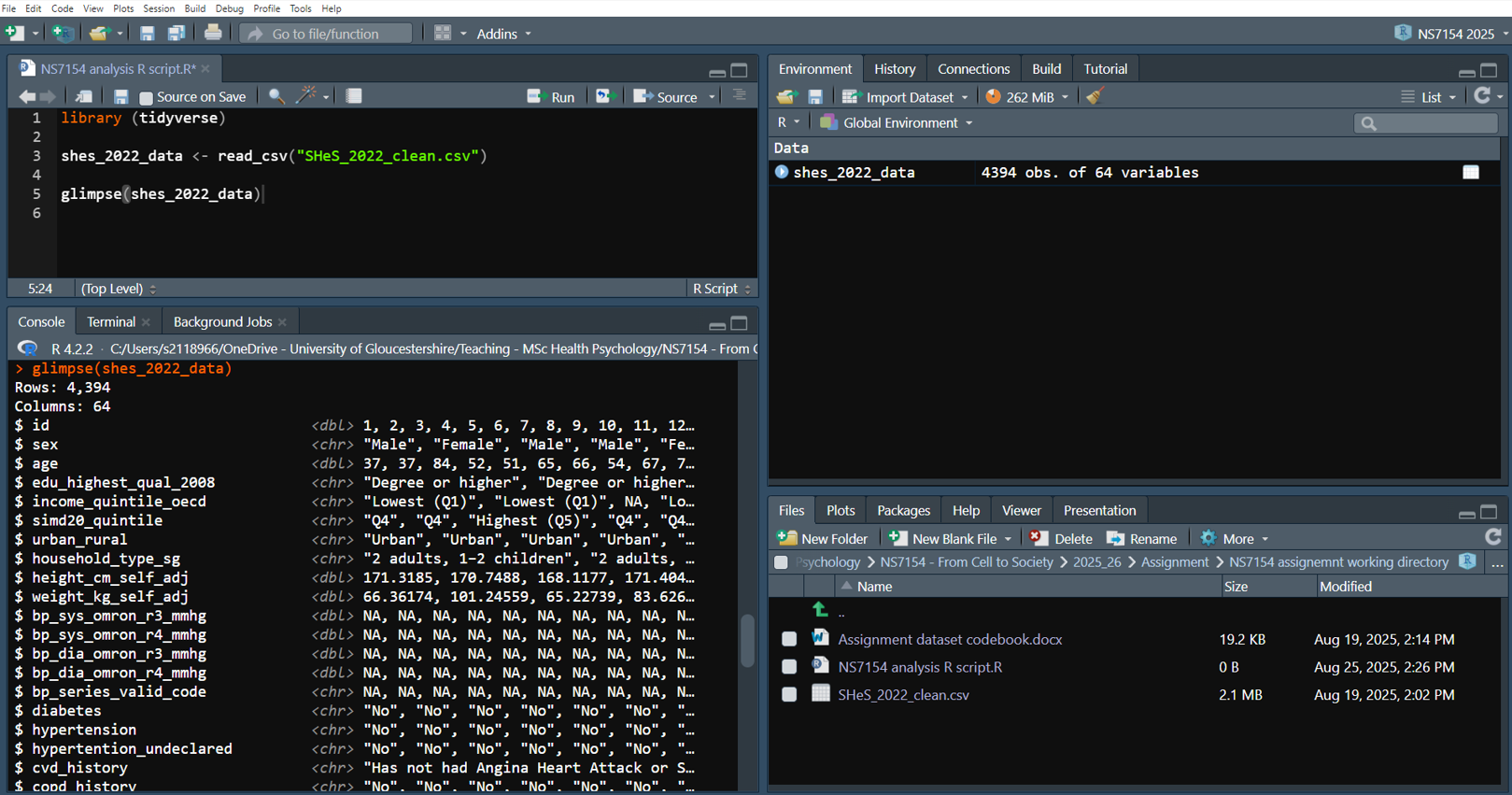
If you’ve followed all of that then well done! This is often the steepest part of the R learning curve. Many people will have tried to learn R and given up due to issues importing their data.
To finish today, we’ll make a smaller dataset with just the variables we need and then create a new variable. We’ll use two tidyverse functions:
select() to pick columns we care about, andmutate() to add new columns (or transform existing ones).Our goal: calculate the Body Mass Index (BMI) for each participant.
shes_BMI <- shes_2022_data %>%
  select(id, height_cm_self_adj, weight_kg_self_adj)
Here is whats happening in the code above:
shes_bmi <- We’re saving the result of what we do next to a new object called shes_bmi.
shes_2022_data %>% Read this as “take shes_2022_data” the %>%, known as a “pipe”, simply reads as “and then…”. The pipe (sometimes written as |> too) passes the data into the next function.
select(id, height_cm_self_adj, weight_kg_self_adj). This keeps only the columns we mention. We have 64 variables in the original. Fewer columns is going to mean less scrolling and fewer chances of us making mistakes.
Next we can perform the calculation to get BMI. The formula we need to follow for this is:
\[ \mathrm{BMI} = \frac{\text{weight (kg)}}{[\text{height (m)}]^2} \]
For the calculation we need to use the mutate() function. This function makes a new variable in a data object.
The height variable seems to be in centimeters so we’ll first create a variable of height in meters. To do this we will need to divide every value in the height_cm_self_adj by 100.
shes_BMI <- shes_BMI %>%
  mutate(height_m = height_cm_self_adj / 100)
Notice with the above code we are writing over the old object with the new object we created. This is fine in this case as all we’re doing is adding a new variable but be extra careful when using other functions just in case you write over your full dataset by accident.
Note also with the mutate() function the new variable name comes first and then that is = to what ever manipulation you want to apply.
The dataset didn’t come with a clear ID number for each participant, so when cleaning, I created one using the the following mutate function.
# creates a variable call id that includes numbers from 1 to 4394
shes_clean <- shes_raw_data %>%
  mutate(id = 1:4394)
The following is a neater way I could do this. Just in case I misread how many observations are in the data object.
shes_clean <- shes_2022_data %>%
  mutate(id2 = row_number())
To finish of the BMI calculation we can conduct another mutate() this time including our newly made height in meters variable.
shes_BMI <- shes_BMI %>%
  mutate(bmi = weight_kg_self_adj / (height_m ^ 2))
The above is an absolutely fine way to create the BMI variable, but the nice thing about R is that you can always tidy up your code to make it neater.
shes_BMI <- shes_2022_data %>%
  select(id, height_cm_self_adj, weight_kg_self_adj) %>%
  mutate(height_m = height_cm_self_adj / 100) %>%
  mutate(bmi = weight_kg_self_adj / (height_m ^ 2))
The above code:
Assigns to a new data object, and then (remember that’s what a %>% mean)
Selects id, height and weight, and then
Creates a height in meters variable by deviding our height in cm variable by 100, and then
Creates our BMI variable using our original weight variable and our new height variable
Can you find a ever more efficient way to calculate BMI?
Tip: Try writing the above expression with just one mutate function.
shes_BMI <- shes_2022_data %>%
  select(id, height_cm_self_adj, weight_kg_self_adj) %>%
    mutate(bmi = weight_kg_self_adj / ((height_cm_self_adj / 100) ^ 2))
Finally, let’s just check that our BMI variable looks correct by creating a quick and easy histogram using the following code:
hist(shes_BMI$bmi)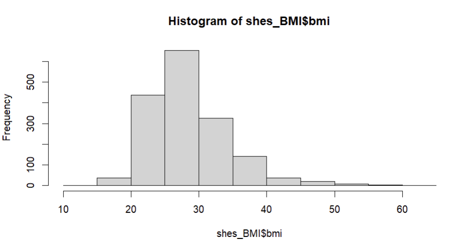 We’ll make much nicer, customisable, figures with the
 ggplot package in session three. But for now this give us a glimpse of our data distribution and shows us that its roughly normally distributed and within the appropriate range for BMI.
The $ in the above code simple tells us to look in the shes_BMI data object and find the variable bmi.
Its from base R rather than tidyverse so you might see it in some older R guides more often.
The final thing to do is to tidy up our code, annotate it (using # comments), and save the script so that we can use the code again in the future. Here is a neat version that will run from the start to finish, so long as the working directory is set correctly, and the directory contains the same .csv file.
# this loads my packages
library(tidyverse)

# this reads in the data
shes_2022_data <- read_csv("SHeS_2022_clean.csv")

# this selects my variables of interest and calculates BMI
shes_BMI <- shes_2022_data %>%
  select(id, height_cm_self_adj, weight_kg_self_adj) %>%
  mutate(bmi = weight_kg_self_adj / ((height_cm_self_adj / 100) ^ 2))

# this creates a simple histogram of BMI
hist(shes_BMI$bmi)Over to you now.
There are two psychometric scales in the dataset these are the Warwick-Edinburgh Mental Wellbeing Scale (WEMWBS) and the General Health Questionnaire (GHQ-12)
See if you can use the select() and mutate() functions to score these up into their latent variables (i.e. combine all items into a single score for each)
Check the codebook for further details related to these scales.
The GHQ-12 will require some thought as some of the items are reverse coded.
Below are how I’d write code to do each of these. But there are many ways to be equally correct when writing code. If you get the same histogram then your way works fine too.
Good luck! And try not to look at the solution until you give it a go for yourself first.
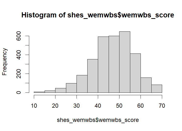
When scored the histogram for the WEMWBS should look like this:
A-ha, caught you (maybe)! You can’t just give up, take my code every time and learn nothing.
Have you tried and failed multiple times? If not, try a few more times. If you’ve hit an error see if you can spot where you’ve gone wrong.
The real solution box can be found at the end of the page.
Now try GHQ-12.
When reverse coding a four point Likert Scale we need 1=4, 2=3, 3=2, 4=1. We could do this with some form of lengthy find and replace, which is likely what you’ve done before when reverse coding variables in SPSS, JASP or Excel.
But a little mathematical trick for this is to take each score away from one higher than the max possible item score. In this case 5 - score = the reverse code. See:
5 - 1 = 45 - 2 = 35 - 3 = 25 - 4 = 1So 5 - variable name will reverse score that variable.
Neat, right!?
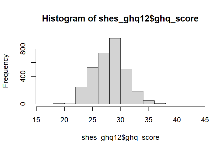
When scored the histogram of the GHQ-12 should look like this:
shes_ghq12 <- shes_2022_data %>%
  select(id, ghqconc, ghqsleep, ghquse, ghqdecis, ghqstrai, ghqover,
         ghqenjoy, ghqface, ghqconfi, ghqworth, ghqunhap, ghqhappy) %>%
  mutate(ghqconcR = 5-ghqconc,
         ghquseR = 5-ghquse,
         ghqdecisR = 5-ghqdecis,
         ghqenjoyR = 5-ghqenjoy,
         ghqfaceR = 5-ghqface,
         ghqhappyR = 5-ghqhappy) %>%
  mutate(ghq_score = ghqconcR + ghqsleep + ghquseR + ghqdecisR + ghqstrai +
           ghqover + ghqenjoyR + ghqfaceR + ghqconfi + ghqworth + ghqunhap +
           ghqhappyR)

hist(shes_ghq12$ghq_score)
This can be reduced down, but I’d feel more comfortable writing this out long hand as it makes it obvious which variables we’ve recoded.
The actual solution for exercise 1 (for real this time):
The following code selects the relevant WEMWBS variables and creates a new variable that is the sum of all the WEMWBS variables.
shes_wemwbs <- shes_2022_data %>%
  select(id, wemwbs_optimistic, wemwbs_useful, wemwbs_relaxed,
         wemwbs_interested_in_people, wemwbs_energy, wemwbs_dealing_problems,
         wemwbs_thinking_clearly, wemwbs_good_about_self, wemwbs_close_to_others,
         wemwbs_confident, wemwbs_make_up_mind, wemwbs_loved,
         wemwbs_interested_in_new_things, wemwbs_cheerful) %>%
  mutate(wemwbs_score = wemwbs_optimistic + wemwbs_useful + wemwbs_relaxed +
         wemwbs_interested_in_people + wemwbs_energy + wemwbs_dealing_problems +
         wemwbs_thinking_clearly + wemwbs_good_about_self + wemwbs_close_to_others +
         wemwbs_confident + wemwbs_make_up_mind + wemwbs_loved + wemwbs_interested_in_new_things +
         wemwbs_cheerful)

hist(shes_wemwbs$wemwbs_score) # check with a histogram
Or, seeing as our variables are labelled in a logical way, a more efficient way to do the same thing would something like:
shes_wemwbs2 <- shes_2022_data %>%
  select(id, starts_with("wemwbs_")) %>%
  mutate(wemwbs_score = rowSums(across(starts_with("wemwbs_"))))

hist(shes_wemwbs2$wemwbs_score) # check with a histogram
But don’t forget we want to priorities readable code over fancy code. If you don’t understanding it rewrite in a longer way that you do understand!
NS7154 Handbook by Dr Richard
Clarke - University of Gloucestershire - rclarke8@glos.ac.uk
Special thanks to Llivia Hales for
editing, testing, and session support!